稀疏性限制

刚才的论述是基于隐藏神经元数量较小的假设。但是即使隐藏神经元的数量较大（可能比输入像素的个数还要多），我们仍然通过给自编码神经网络施加一些其他的限制条件来发现输入数据中的结构。具体来说，如果我们给隐藏神经元加入稀疏性限制，那么自编码神经网络即使在隐藏神经元数量较多的情况下仍然可以发现输入数据中一些有趣的结构。 
稀疏性可以被简单地解释如下。如果当神经元的输出接近于1的时候我们认为它被激活，而输出接近于0的时候认为它被抑制，那么使得神经元大部分的时间都是被抑制的限制则被称作稀疏性限制。这里我们假设的神经元的激活函数是sigmoid函数。如果你使用tanh作为激活函数的话，当神经元输出为-1的时候，我们认为神经元是被抑制的。

何必为难它呢？为什么要让只要少部分中间隐藏神经元的活跃度，也就是输出值大于0，其他的大部分为0.原因就是我们要做的就是模拟我们人脑。神经网络本来就是模型人脑神经元的，深度学习也是。在人脑中有大量的神经元，但是大多数自然图像通过我们视觉进入人脑时，只会刺激到少部分神经元，而大部分神经元都是出于抑制状态的。而且，大多数自然图像，都可以被表示为少量基本元素（面或者线）的叠加。又或者说，这样更加有助于我们用少量的神经元提取出自然图像更加本质的特征。

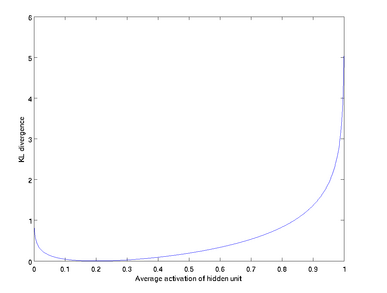
由上图可以看到，当 p′j=p 的时候，∑s2j=1KL(p||p′j) 的值为0，而当 p′j 远离 p 的时候，∑s2j=1KL(p||p′j) 的值快速增大。因此，很明显，这个惩罚因子的作用就是让 p′j 尽可能靠近 p ,从而达到我们的稀疏性限制。更加具体的计算，请参考ULFDL。

Matlab 实战

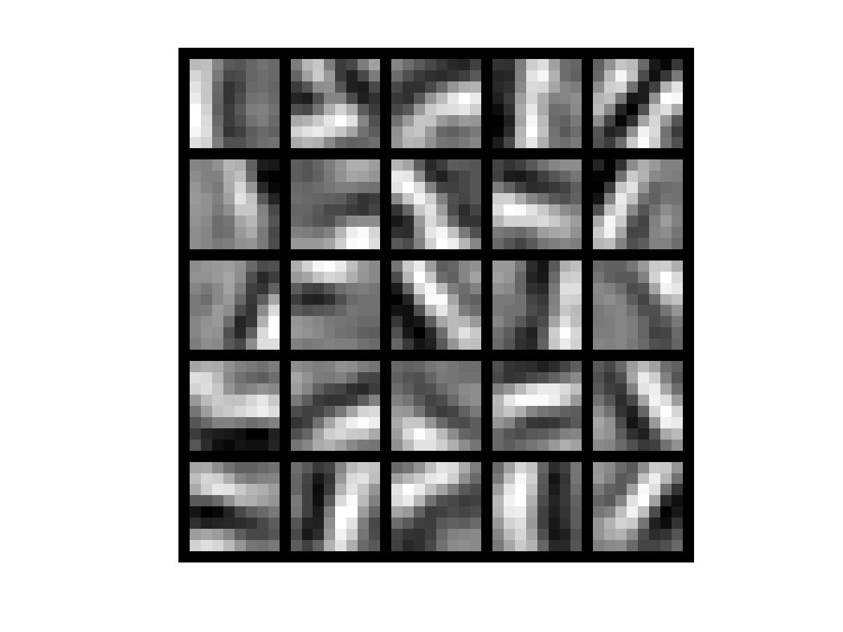
这里的输入数据是 8x8 的一个小图片，转换为 64x1 的矩阵，总共10000个样本进行训练，学习图片中的特征，其实结果就是图片的边缘。效果如下图：

代码如下：sparseAutoencoderCost.m

function [cost,grad] = sparseAutoencoderCost(theta, visibleSize, hiddenSize, ...
                                             lambda, sparsityParam, beta, data)
%lambda = 0;
%beta = 0;
% visibleSize: the number of input units (probably 64) 
% hiddenSize: the number of hidden units (probably 25) 
% lambda: weight decay parameter
% sparsityParam: The desired average activation for the hidden units (denoted in the lecture
%                           notes by the greek alphabet rho, which looks like a lower-case "p").
% beta: weight of sparsity penalty term
% data: Our 64x10000 matrix containing the training data.  So, data(:,i) is the i-th training example. 

% The input theta is a vector (because minFunc expects the parameters to be a vector). 

% We first convert theta to the (W1, W2, b1, b2) matrix/vector format, so that this 
% follows the notation convention of the lecture notes. 

% 学习率 自己定义的
alpha = 0.01;

% 隐藏神经元的个数是   25   = hiddenSize

% 计算隐藏层神经元的激活度
p = zeros(hiddenSize,1);

% 25x64
W1 = reshape(theta(1:hiddenSize*visibleSize), hiddenSize, visibleSize);
% 64 X 25
W2 = reshape(theta(hiddenSize*visibleSize+1:2*hiddenSize*visibleSize), visibleSize, hiddenSize);
% 25 X1
b1 = theta(2*hiddenSize*visibleSize+1:2*hiddenSize*visibleSize+hiddenSize);
% 64 x 1
b2 = theta(2*hiddenSize*visibleSize+hiddenSize+1:end);

% Cost and gradient variables (your code needs to compute these values). 
% Here, we initialize them to zeros. 

% costFunction 的第一项
%{
J_sparse = 0;
W1grad = zeros(size(W1)); 
W2grad = zeros(size(W2));
b1grad = zeros(size(b1)); 
b2grad = zeros(size(b2));
%}
%% ---------- YOUR CODE HERE --------------------------------------
%  Instructions: Compute the cost/optimization objective J_sparse(W,b) for the Sparse Autoencoder,
%                and the corresponding gradients W1grad, W2grad, b1grad, b2grad.
%
% W1grad, W2grad, b1grad and b2grad should be computed using backpropagation.
% Note that W1grad has the same dimensions as W1, b1grad has the same dimensions
% as b1, etc.  Your code should set W1grad to be the partial derivative of J_sparse(W,b) with
% respect to W1.  I.e., W1grad(i,j) should be the partial derivative of J_sparse(W,b) 
% with respect to the input parameter W1(i,j).  Thus, W1grad should be equal to the term 
% [(1/m) \Delta W^{(1)} + \lambda W^{(1)}] in the last block of pseudo-code in Section 2.2 
% of the lecture notes (and similarly for W2grad, b1grad, b2grad).
% 
% Stated differently, if we were using batch gradient descent to optimize the parameters,
% the gradient descent update to W1 would be W1 := W1 - alpha * W1grad, and similarly for W2, b1, b2. 
% 


% 批量梯度下降法的一次迭代  data 64x10000
numPatches = size(data,2);
KLdist = 0;

% 25x10000
%a2 = zeros(size(W1,1),numPatches);
% 64x10000
%a3 = zeros(size(W2,1),numPatches);

%% 向前传输
% 25x10000  25x64 64x10000 
a2 = sigmoid(W1*data+repmat(b1,[1,numPatches]));
p = sum(a2,2);
a3 = sigmoid(W2 * a2 + repmat(b2,[1,numPatches]));
J_sparse = 0.5 * sum(sum((a3-data).^2));

%{
for curPatch = 1:numPatches

    % 计算激活值   
    % 25 X1 第二层的激活值   25x64  64x1
    a2(:,curPatch) = sigmoid(W1 * data(:,curPatch) + b1);
    % 计算隐藏层神经元的总激活值
    p = p + a2(:,curPatch); 
    % 64 x1 第三层的激活值
    a3(:,curPatch) = sigmoid(W2 * a2(:,curPatch) +b2);    
    %  计算costFunction的第一项
    J_sparse = J_sparse + 0.5 * (a3(:,curPatch)-data(:,curPatch))' * (a3(:,curPatch)-data(:,curPatch)) ;
end
%}

%% 计算 隐藏层的平均激活度
p = p /  numPatches ;

%% 向后传输 

 %64x10000
    residual3 = -(data-a3).*a3.*(1-a3);
    %25x10000
    tmp = beta * ( - sparsityParam ./ p + (1-sparsityParam) ./ (1-p));
    %  25x10000   25x64 64x10000  
    residual2 = (W2' * residual3 + repmat(tmp,[1,numPatches])) .* a2.*(1-a2);
    W2grad = residual3 * a2' / numPatches + lambda * W2 ;
    W1grad = residual2 * data'  / numPatches + lambda * W1 ;
    b2grad = sum(residual3,2) / numPatches; 
    b1grad = sum(residual2,2) / numPatches; 

    %{
for curPatch = 1:numPatches

    %  计算残差  64x1    
   % residual3 = -( data(:,curPatch) - a3(:,curPatch)) .* (a3 - a3.^2);
    residual3 = -(data(:,curPatch) - a3(:,curPatch)).* (a3(:,curPatch) - (a3(:,curPatch).^2));
    %  25x1         25x 64  *  64X1   ==>  25X1  .*   25X1
    residual2 = (W2' * residual3 + beta * (- sparsityParam ./ p + (1-sparsityParam) ./ (1-p))) .* (a2(:,curPatch) - (a2(:,curPatch)).^2);
  %  residual2 = (W2' * residual3 ) .* (a2(:,curPatch) - (a2(:,curPatch)).^2);
    % 计算偏导数值
    %   64 x25   =  64x1    1x25
    W2grad = W2grad + residual3 * a2(:,curPatch)';
    % 64 x1 = 64x1
    b2grad = b2grad + residual3;
    % 25x64  =  25x1  * 1x64
    W1grad = W1grad + residual2 *   data(:,curPatch)';
    % 25x1 = 25x1
    b1grad = b1grad + residual2;
    %J_sparse = J_sparse + (a3 - data(:,curPatch))' * (a3 - data(:,curPatch));

end

W2grad = W2grad / numPatches + lambda * W2;
W1grad = W1grad / numPatches + lambda * W1;
b2grad = b2grad / numPatches;
b1grad = b1grad / numPatches;

 %}

%% 更新权重参数   加上 lambda  权重衰减
W2 = W2 - alpha * ( W2grad  );
W1 = W1 - alpha * ( W1grad );

b2 = b2 - alpha * (b2grad );
b1 = b1 - alpha * (b1grad );

%% 计算KL相对熵
for j = 1:hiddenSize
    KLdist = KLdist + sparsityParam *log( sparsityParam / p(j) )   +   (1 - sparsityParam) * log((1-sparsityParam) / (1 - p(j)));
end

%% costFunction 加上 lambda 权重衰减
cost = J_sparse / numPatches + (sum(sum(W1.^2)) + sum(sum(W2.^2))) * lambda / 2  + beta * KLdist;

%cost = J_sparse / numPatches + (sum(sum(W1.^2)) + sum(sum(W2.^2))) * lambda / 2;


%-------------------------------------------------------------------
% After computing the cost and gradient, we will convert the gradients back
% to a vector format (suitable for minFunc).  Specifically, we will unroll
% your gradient matrices into a vector.

grad = [W1grad(:) ; W2grad(:) ; b1grad(:) ; b2grad(:)];

end

%-------------------------------------------------------------------
% Here's an implementation of the sigmoid function, which you may find useful
% in your computation of the costs and the gradients.  This inputs a (row or
% column) vector (say (z1, z2, z3)) and returns (f(z1), f(z2), f(z3)). 

function sigm = sigmoid(x)
    sigm = 1 ./ (1 + exp(-x));
end
1
2
3
4
5
6
7
8
9
10
11
12
13
14
15
16
17
18
19
20
21
22
23
24
25
26
27
28
29
30
31
32
33
34
35
36
37
38
39
40
41
42
43
44
45
46
47
48
49
50
51
52
53
54
55
56
57
58
59
60
61
62
63
64
65
66
67
68
69
70
71
72
73
74
75
76
77
78
79
80
81
82
83
84
85
86
87
88
89
90
91
92
93
94
95
96
97
98
99
100
101
102
103
104
105
106
107
108
109
110
111
112
113
114
115
116
117
118
119
120
121
122
123
124
125
126
127
128
129
130
131
132
133
134
135
136
137
138
139
140
141
142
143
144
145
146
147
148
149
150
151
152
153
154
155
156
157
158
159
160
161
162
163
164
165
166
167
168
169
170
171
172
173

代码中包含了向量方式实现和非向量方式实现。向量方式实现代码量少，运行速度也很快。代码中注释写得很清楚了，就不说了。

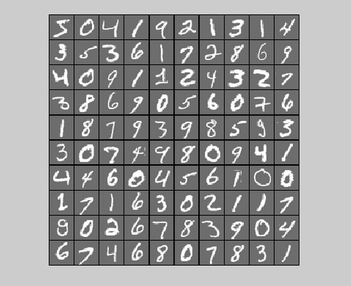
接下来是实现第二个例子，我们将从如下的图像中学习其中包含的特征，这里的输入图像是 28x28 ，隐藏层单元是 196 个，算法使用向量化编程，不然又得跑很久了吼吼吼。

原始图像如下：

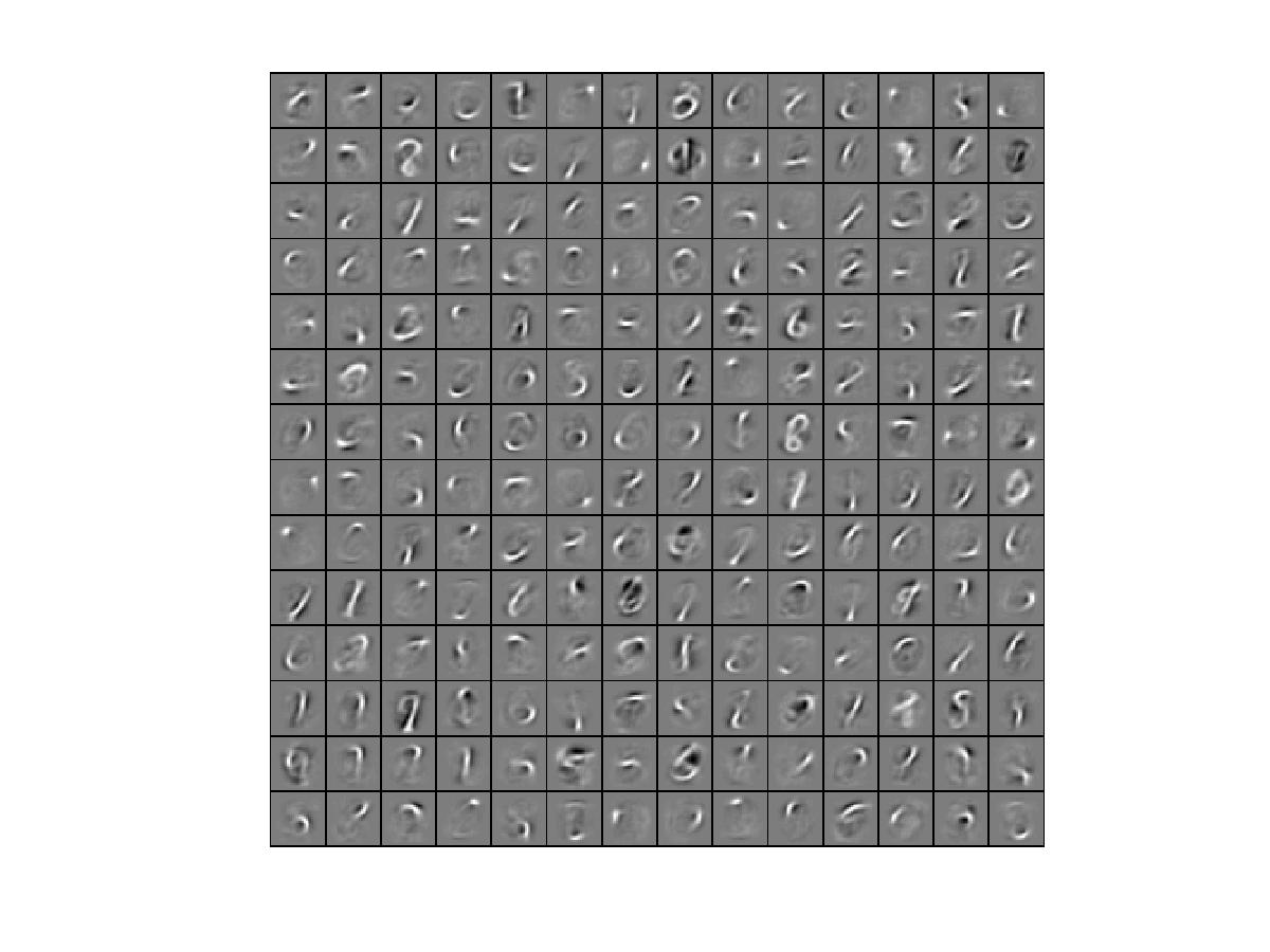
最终学习得到的图像如下：

代码如下：

function [cost,grad] = sparseAutoencoderCost(theta, visibleSize, hiddenSize, ...
                                             lambda, sparsityParam, beta, data)
%lambda = 0;
%beta = 0;
% visibleSize: the number of input units (probably 64) 
% hiddenSize: the number of hidden units (probably 25) 
% lambda: weight decay parameter
% sparsityParam: The desired average activation for the hidden units (denoted in the lecture
%                           notes by the greek alphabet rho, which looks like a lower-case "p").
% beta: weight of sparsity penalty term
% data: Our 64x10000 matrix containing the training data.  So, data(:,i) is the i-th training example. 

% The input theta is a vector (because minFunc expects the parameters to be a vector). 

% We first convert theta to the (W1, W2, b1, b2) matrix/vector format, so that this 
% follows the notation convention of the lecture notes. 

% 学习率 自己定义的
alpha = 0.03;

% 计算隐藏层神经元的激活度
p = zeros(hiddenSize,1);

W1 = reshape(theta(1:hiddenSize*visibleSize), hiddenSize, visibleSize);
W2 = reshape(theta(hiddenSize*visibleSize+1:2*hiddenSize*visibleSize), visibleSize, hiddenSize);
b1 = theta(2*hiddenSize*visibleSize+1:2*hiddenSize*visibleSize+hiddenSize);
b2 = theta(2*hiddenSize*visibleSize+hiddenSize+1:end);

% Cost and gradient variables (your code needs to compute these values). 
% Here, we initialize them to zeros. 

%% ---------- YOUR CODE HERE --------------------------------------
%  Instructions: Compute the cost/optimization objective J_sparse(W,b) for the Sparse Autoencoder,
%                and the corresponding gradients W1grad, W2grad, b1grad, b2grad.
%
% W1grad, W2grad, b1grad and b2grad should be computed using backpropagation.
% Note that W1grad has the same dimensions as W1, b1grad has the same dimensions
% as b1, etc.  Your code should set W1grad to be the partial derivative of J_sparse(W,b) with
% respect to W1.  I.e., W1grad(i,j) should be the partial derivative of J_sparse(W,b) 
% with respect to the input parameter W1(i,j).  Thus, W1grad should be equal to the term 
% [(1/m) \Delta W^{(1)} + \lambda W^{(1)}] in the last block of pseudo-code in Section 2.2 
% of the lecture notes (and similarly for W2grad, b1grad, b2grad).
% 
% Stated differently, if we were using batch gradient descent to optimize the parameters,
% the gradient descent update to W1 would be W1 := W1 - alpha * W1grad, and similarly for W2, b1, b2. 
% 
numPatches = size(data,2);
KLdist = 0;

%% 向前传输

a2 = sigmoid(W1*data+repmat(b1,[1,numPatches]));
p = sum(a2,2);
a3 = sigmoid(W2 * a2 + repmat(b2,[1,numPatches]));
J_sparse = 0.5 * sum(sum((a3-data).^2));

%% 计算 隐藏层的平均激活度
p = p /  numPatches ;

%% 向后传输 

    residual3 = -(data-a3).*a3.*(1-a3);
    tmp = beta * ( - sparsityParam ./ p + (1-sparsityParam) ./ (1-p));
    residual2 = (W2' * residual3 + repmat(tmp,[1,numPatches])) .* a2.*(1-a2);

    W2grad = residual3 * a2' / numPatches + lambda * W2 ;
    W1grad = residual2 * data'  / numPatches + lambda * W1 ;
    b2grad = sum(residual3,2) / numPatches; 
    b1grad = sum(residual2,2) / numPatches; 

%% 更新权重参数   加上 lambda  权重衰减
W2 = W2 - alpha * ( W2grad  );
W1 = W1 - alpha * ( W1grad );

b2 = b2 - alpha * (b2grad );
b1 = b1 - alpha * (b1grad );

%% 计算KL相对熵
for j = 1:hiddenSize
    KLdist = KLdist + sparsityParam *log( sparsityParam / p(j) )   +   (1 - sparsityParam) * log((1-sparsityParam) / (1 - p(j)));
end

%% costFunction 加上 lambda 权重衰减
cost = J_sparse / numPatches + (sum(sum(W1.^2)) + sum(sum(W2.^2))) * lambda / 2  + beta * KLdist;

%-------------------------------------------------------------------
% After computing the cost and gradient, we will convert the gradients back
% to a vector format (suitable for minFunc).  Specifically, we will unroll
% your gradient matrices into a vector.

grad = [W1grad(:) ; W2grad(:) ; b1grad(:) ; b2grad(:)];

end

%-------------------------------------------------------------------
% Here's an implementation of the sigmoid function, which you may find useful
% in your computation of the costs and the gradients.  This inputs a (row or
% column) vector (say (z1, z2, z3)) and returns (f(z1), f(z2), f(z3)). 

function sigm = sigmoid(x)

    sigm = 1 ./ (1 + exp(-x));
end