【Python机器学习系列】一文教你建立随机森林-贝叶斯优化模型预测房价(案例+源码)
一文教你建立随机森林-贝叶斯优化模型预测房价(案例+源码)
这是我的第446篇原创文章。
一、引言
本文用回归数据训练RandomForestRegressor,用贝叶斯优化(SMBO 或 PyTorch NN;acquisition = Expected Improvement)在有限评估预算下高效搜索超参数。最终比随机搜索在少量评估下更快找到更好的超参数组合。并用可视化说明优化轨迹、surrogate 预测、EI 分布及最终预测效果等关键点。我们要优化的函数:超参数 => 验证集分数(或 CV 分数)。每次评估很耗时(训练 RF),所以要少做训练但尽量找到好参数。
贝叶斯优化用代理模型(surrogate)来估计目标函数,并用采集函数决定下一个最值得评估的超参数点(EI、PI、UCB等)。代理模型既可以是 GP,也可以是树,也可以是 NN。我们用随机森林作为代理(兼容类别参数、稳健、扩展性好),另提供 PyTorch NN 代理做对比。用采集函数(EI)在代理预测均值与不确定性上折衷“探索 vs 利用”。
二、实现过程
2.1 读取数据
核心代码:
def read_data(filename):
filename = filename
names = ['CRIM', 'ZN', 'INDUS', 'CHAS', 'NOX', 'RM', 'AGE', 'DIS',
'RAD', 'TAX', 'PRTATIO', 'B', 'LSTAT', 'MEDV']
dataset = pd.read_csv(filename, names=names, delim_whitespace=True)
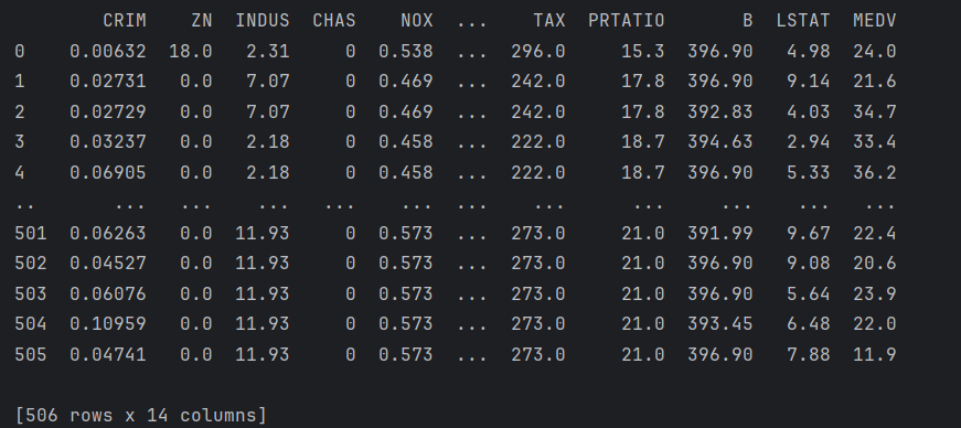
print(dataset)
df = pd.DataFrame(dataset)
# 划分数据集
features = names[:-1]
X = df[features].values
y = df['MEDV'].values
return X, y
X, y = read_data('data.csv')结果:
2.2 数据划分与归一化
核心代码:
X_train_full, X_test, y_train_full, y_test = train_test_split(X, y, test_size=0.2, random_state=seed)
X_train, X_val, y_train, y_val = train_test_split(X_train_full, y_train_full, test_size=0.2, random_state=seed)
scaler = StandardScaler()
X_train = scaler.fit_transform(X_train)
X_val = scaler.transform(X_val)
X_test = scaler.transform(X_test)
2.3 运行BO
核心代码:
def bayes_optimize_rf(X_train, y_train, X_val, y_val,
                      n_init=10, n_iter=40, surrogate_type='rf', random_seed=0,
                      candidate_pool_size=1000):
    """
    surrogate_type: 'rf' or 'torch'
    返回:history 列表,包含 (params, score, time)
    """
    rng = check_random_state(random_seed)
    # 数据容器
    vectors = []
    y_vals = []  # 我们用目标是 r2,若需要最小化 mse,可改
    params_list = []
    history = []
    # 初始随机点
    init_params = sample_random_params(rng, n_init)
    for p in init_params:
        res = evaluate_rf(X_train, y_train, X_val, y_val, p, random_state=random_seed)
        score = res['r2']  # 我们最大化 r2
        vectors.append(params_to_vector(p))
        y_vals.append(score)
        params_list.append(p)
        history.append({'params': p, 'r2': score, 'mse': res['mse']})
    best_idx = int(np.argmax(y_vals))
    best_score = y_vals[best_idx]
    best_params = params_list[best_idx].copy()
    for it in range(n_iter):
        # train surrogate on existing (vectors, y_vals)
        Xs = np.vstack(vectors)
        ys = np.array(y_vals)
        if surrogate_type == 'rf':
            # surrogate predicts mean by RF; to get sigma we use tree-wise predictions variance
            surf = RandomForestRegressor(n_estimators=200, n_jobs=-1, random_state=random_seed)
            surf.fit(Xs, ys)
            # candidate pool
            cands = sample_random_params(rng, n_samples=candidate_pool_size)
            cvecs = np.vstack([params_to_vector(c) for c in cands])
            mu = surf.predict(cvecs)
            # compute "sigma" as std of predictions from individual trees
            all_tree_preds = np.stack([t.predict(cvecs) for t in surf.estimators_], axis=0)  # (n_trees, n_cand)
            sigma = np.std(all_tree_preds, axis=0, ddof=1)
        else:
            # torch surrogate
            surf_model = train_torch_surrogate(Xs, ys, epochs=400, lr=1e-3, verbose=False)
            cands = sample_random_params(rng, n_samples=candidate_pool_size)
            cvecs = np.vstack([params_to_vector(c) for c in cands])
            mu, sigma = predict_torch_mc(surf_model, cvecs, n_samples=60)
        # compute EI (maximize)
        f_best = best_score
        ei = expected_improvement(mu, sigma, f_best, xi=0.01)
        # select best candidate
        idx_best = int(np.argmax(ei))
        cand_params = cands[idx_best]
        # evaluate real objective
        t0 = time.time()
        res = evaluate_rf(X_train, y_train, X_val, y_val, cand_params, random_state=random_seed)
        t1 = time.time()
        score = res['r2']
        # append
        vectors.append(params_to_vector(cand_params))
        y_vals.append(score)
        params_list.append(cand_params)
        history.append({'params': cand_params, 'r2': score, 'mse': res['mse'], 'time': t1 - t0})
        # update best
        if score > best_score:
            best_score = score
            best_params = cand_params.copy()
        # debug print
        print(f"Iter {it+1}/{n_iter} - cand best EI idx {idx_best}, r2={score:.4f}, best_r2={best_score:.4f}")
    return {'history': history, 'best_score': best_score, 'best_params': best_params}
贝叶斯优化主流程(surrogate = sklearn RF or PyTorch surrogate)
- 初始随机采样 n_init
- 每轮:训练 surrogate,产生一大批候选点(随机采样),用 surrogate 预测 mu/sigma,计算 EI,选择最大 EI 的点去真实评估
- 记录轨迹(每次最好分数、最佳超参)
随机森林 surrogate,用来拟合超参数空间->得分
- 我们用 RandomForestRegressor 作为 surrogate(回归目标为验证 MSE 或 -r2)
- 并用随机候选优化采集函数(采样一批候选点,用 surrogate 估计 EI,然后挑选最优)
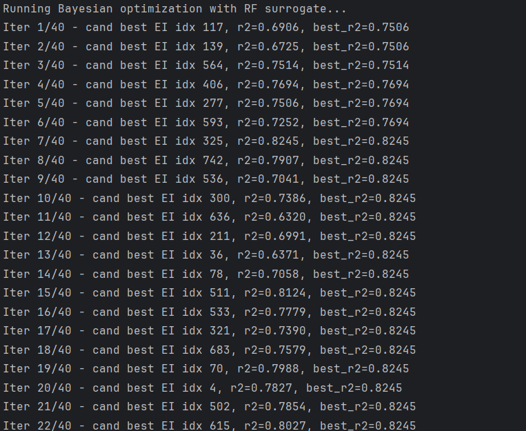
bo_rf = bayes_optimize_rf(X_train, y_train, X_val, y_val,
                          n_init=n_init, n_iter=n_iter, surrogate_type='rf', random_seed=seed,
                          candidate_pool_size=800)
结果:
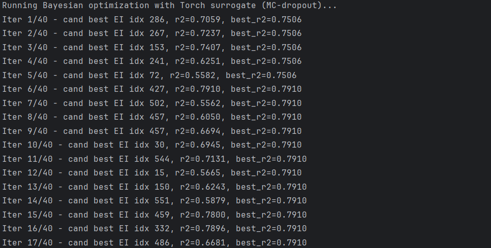
PyTorch surrogate:一个小 MLP + MC-dropout,用来估计预测均值和不确定度,训练方式:最小二乘,预测时多次前向取均值和方差)
bo_torch = bayes_optimize_rf(X_train, y_train, X_val, y_val,
                             n_init=n_init, n_iter=n_iter, surrogate_type='torch', random_seed=seed,
                             candidate_pool_size=600)
结果:
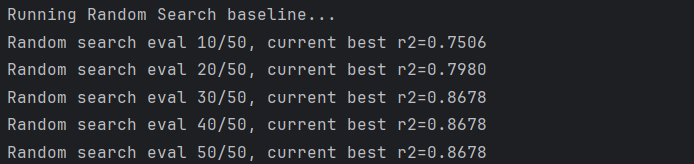
2.4 对照:随机搜索 baseline(相同评估次数)
核心代码:
def random_search_rf(X_train, y_train, X_val, y_val, n_evals=50, random_seed=0):
    rng = check_random_state(random_seed)
    history = []
    best_score = -np.inf
    best_params = None
    for i in range(n_evals):
        p = sample_random_params(rng, 1)[0]
        res = evaluate_rf(X_train, y_train, X_val, y_val, p, random_state=random_seed)
        score = res['r2']
        history.append({'params': p, 'r2': score, 'mse': res['mse']})
        if score > best_score:
            best_score = score
            best_params = p.copy()
        if (i+1) % 10 == 0:
            print(f"Random search eval {i+1}/{n_evals}, current best r2={best_score:.4f}")
    return {'history': history, 'best_score': best_score, 'best_params': best_params}
结果:
2.5 测试集评估
核心代码:
test_res_bo_rf = eval_on_test(bo_rf['best_params'])
test_res_bo_torch = eval_on_test(bo_torch['best_params'])
test_res_rs = eval_on_test(rs['best_params'])
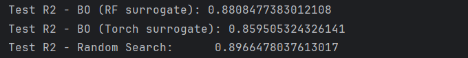
print("Test R2 - BO (RF surrogate):", test_res_bo_rf['r2'])
print("Test R2 - BO (Torch surrogate):", test_res_bo_torch['r2'])
print("Test R2 - Random Search: ", test_res_rs['r2'])结果:
2.6 数据分析可视化
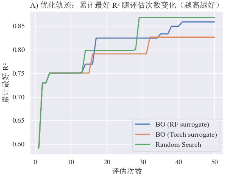
A) 优化轨迹:每次评估的 best R2 随评估次数变化(对比 BO_rf, BO_torch, RS)
核心代码:
bo_rf = exp_res['bo_rf']
bo_torch = exp_res['bo_torch']
rs = exp_res['rs']
X_test = exp_res['X_test']; y_test = exp_res['y_test']
# A: 优化轨迹(累计最好 r2)
def cum_best(history):
    bests = []
    cur_best = -np.inf
    for h in history:
        cur_best = max(cur_best, h['r2'])
        bests.append(cur_best)
    return np.array(bests)
hist_bo_rf = bo_rf['history']
hist_bo_torch = bo_torch['history']
hist_rs = rs['history']
cum_rf = cum_best(hist_bo_rf)
cum_torch = cum_best(hist_bo_torch)
cum_rs = cum_best(hist_rs)
eval_idx_rf = np.arange(1, len(cum_rf)+1)
eval_idx_torch = np.arange(1, len(cum_torch)+1)
eval_idx_rs = np.arange(1, len(cum_rs)+1)
plt.plot(eval_idx_rf, cum_rf, label='BO (RF surrogate)', linewidth=2)
plt.plot(eval_idx_torch, cum_torch, label='BO (Torch surrogate)', linewidth=2)
plt.plot(eval_idx_rs, cum_rs, label='Random Search', linewidth=2)
plt.title("A) 优化轨迹:累计最好 R² 随评估次数变化(越高越好)")
plt.xlabel("评估次数")
plt.ylabel("累计最好 R²")
plt.legend()
plt.show()
结果:累计最好 R² 随评估次数的变化,直观对比在相同评估次数下哪种策略更快地提升性能(样本效率)。若 BO 相比随机搜索更陡峭则说明高效性。
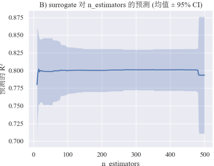
B) surrogate :在参数空间上的预测 vs 真实观察(用第一个参数 n_estimators 做一维切片示意)
核心代码:
all_vecs_rf = np.vstack([params_to_vector(h['params']) for h in hist_bo_rf])
all_scores_rf = np.array([h['r2'] for h in hist_bo_rf])
surf_final = RandomForestRegressor(n_estimators=300, random_state=0)
surf_final.fit(all_vecs_rf, all_scores_rf)
# vary n_estimators while holding others fixed at median
med_vec = np.median(all_vecs_rf, axis=0)
n_grid = np.linspace(param_space['n_estimators'][0], param_space['n_estimators'][1], 200)
grid_vecs = []
for n in n_grid:
    v = med_vec.copy()
    v[0] = n
    grid_vecs.append(v)
grid_vecs = np.vstack(grid_vecs)
mu_grid = surf_final.predict(grid_vecs)
# get predictions from each tree to estimate sigma
all_tree_preds = np.stack([t.predict(grid_vecs) for t in surf_final.estimators_], axis=0)
sigma_grid = np.std(all_tree_preds, axis=0, ddof=1)
plt.plot(n_grid, mu_grid, linestyle='-', linewidth=2)
plt.fill_between(n_grid, mu_grid - 1.96*sigma_grid, mu_grid + 1.96*sigma_grid, alpha=0.25)
plt.title("B) surrogate 对 n_estimators 的预测 (均值 ± 95% CI)")
plt.xlabel("n_estimators")
plt.ylabel("预测的 R²")
plt.show()
结果:surrogate 对n_estimators的 1D 切片预测(均值 ± 95% 置信区间)。 surrogate 如何在参数轴上预测性能趋势与不确定性,以及模型认为哪些 n_estimators 值可能更好。
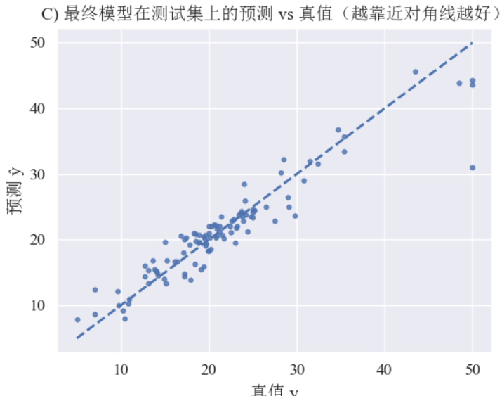
C) 最终模型在测试集上的预测 vs 真值(预测曲线)
核心代码:
best_params_rf = bo_rf['best_params']
final_rf_model = RandomForestRegressor(
    n_estimators=int(best_params_rf['n_estimators']),
    max_depth=None if best_params_rf['max_depth'] is None else int(best_params_rf['max_depth']),
    min_samples_split=int(best_params_rf['min_samples_split']),
    min_samples_leaf=int(best_params_rf['min_samples_leaf']),
    max_features=best_params_rf['max_features'],
    random_state=0, n_jobs=-1, bootstrap=best_params_rf['bootstrap']
)
X_train_comb = np.vstack([exp_res['X_train'], exp_res['X_val']])
y_train_comb = np.concatenate([exp_res['y_train'], exp_res['y_val']])
final_rf_model.fit(X_train_comb, y_train_comb)
y_pred_test = final_rf_model.predict(X_test)
# sort by true y for a cleaner curve
idx = np.argsort(y_test)
plt.scatter(y_test[idx], y_pred_test[idx], s=12, alpha=0.8)
# plot ideal line
mn = min(y_test.min(), y_pred_test.min()); mx = max(y_test.max(), y_pred_test.max())
plt.plot([mn, mx], [mn, mx], linestyle='--', linewidth=2)
plt.title("C) 最终模型在测试集上的预测 vs 真值(越靠近对角线越好)")
plt.xlabel("真值 y")
plt.ylabel("预测 ŷ")
plt.show()
结果:最终模型在测试集上的预测 vs 真值(散点图 + 对角线),最终模型泛化效果,点越接近对角线说明拟合越好。
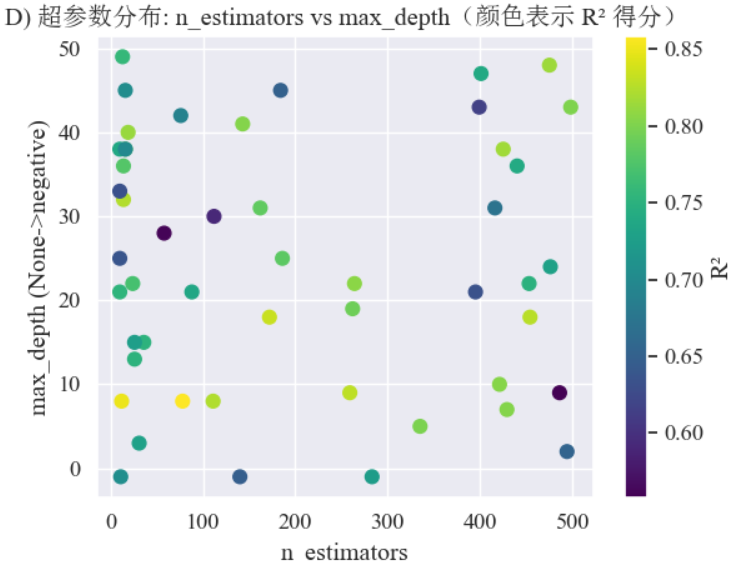
D) 超参数散点图:展示评估点在两个重要参数维度上的分布及其得分(彩色可视化)
核心代码:
param_points = np.array([params_to_vector(h['params']) for h in hist_bo_rf])
scores = np.array([h['r2'] for h in hist_bo_rf])
fig, ax3 = plt.subplots()
sc = plt.scatter(param_points[:, 0], param_points[:, 1], c=scores, s=60, cmap='viridis')
ax3.set_title("D) 超参数分布: n_estimators vs max_depth(颜色表示 R² 得分)")
ax3.set_xlabel("n_estimators")
ax3.set_ylabel("max_depth (None->negative)")
cbar = fig.colorbar(sc, ax=ax3)
cbar.set_label('R²')
ax3.grid(True)
plt.show()
结果:超参数散点图,可视化 BO 在参数空间里的探索轨迹,颜色表示表现如何,有助观察是否在某一区域集中找到好参数。
作者简介:
读研期间发表6篇SCI数据挖掘相关论文,现在某研究院从事数据算法相关科研工作,结合自身科研实践经历不定期分享关于Python、机器学习、深度学习、人工智能系列基础知识与应用案例。致力于只做原创,以最简单的方式理解和学习,关注我一起交流成长。需要数据集和源码的小伙伴可以关注底部公众号添加作者微信。

脑启社区是一个专注类脑智能领域的开发者社区。欢迎加入社区,共建类脑智能生态。社区为开发者提供了丰富的开源类脑工具软件、类脑算法模型及数据集、类脑知识库、类脑技术培训课程以及类脑应用案例等资源。
更多推荐


 28
28 0
0- 0


 已为社区贡献1条内容

所有评论(0)