一、注意力机制

自主性的与非自主性的注意力提示解释了人类的注意力的方式，下面来看看如何通过这两种注意力提示，用神经网络来设计注意力机制的框架：

  首先，考虑一个相对简单的状况，即只使用非自主性提示。要想将选择偏向于感官输入，则可以简单地使用参数化的全连接层，甚至是非参数化的最大汇聚层或平均汇聚层。因此，“是否包含自主性提示”将注意力机制与全连接层或汇聚层区别开来。

卷积、全连接层、汇聚层通常只考虑不随意线索，因为它们都暴力地将所有数据都直接输入到神经网络中，而不对目标加以区分。

注意力机制则考虑随意线索。

在注意力机制中，自主性提示被称为查询（query），而非自主性提示（客观存在的咖啡杯和书本）作为键（key）与感官输入（sensory inputs）的值（value）构成一组 pair 作为输入。而给定任何查询，注意力机制通过注意力汇聚（attention pooling）将非自主性提示的 key 引导至感官输入。如下图所示，可以通过设计注意力汇聚的方式，便于给定的查询（自主性提示）与键（非自主性提示）进行匹配，这将引导得出最匹配的值（感官输入）：

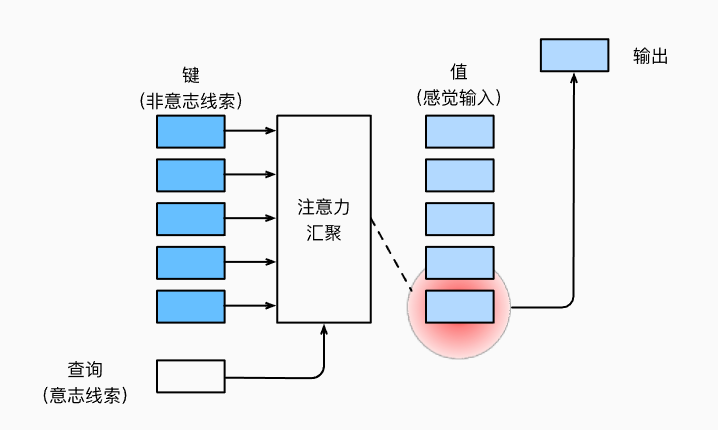
例如，在侦探工作中，每个线索都由一个属性（key）和其价值（value）组成。这些线索可能包括目击者证词、凶器、不在场证明等，而它们的价值可能各不相同，甚至线索可能会误导调查。 如果我们不采用注意力机制，需要对所有线索进行平等的调查，这导致在不重要的线索上花费过多的时间和精力。数学上，这种做法相当于将所有线索的价值简单相加，由于价值有正有负，最终的总价值可能并不高，无法有效指导我们的调查。 然而，通过使用注意力机制，我们可以更加智能地处理这些线索。首先，我们会计算每个线索的属性（key）与我们当前关注的问题（query）之间的相关性。例如，凶器和目击者证词很可能与破案有很高的相关性。然后，会将与问题高度相关的线索的价值（value）进行加权求和，这样不仅可以保证我们集中精力在最重要的线索上，而且可以提高我们得到有价值信息的可能性。

二、Nadaraya-Watson 核回归

Nadaraya-Watson 核回归（Nadaraya-Watson Kernel Regression）是一种非参数回归方法，用于估计一个目标变量（输出）与一个或多个特征变量（输入）之间的关系。该方法通过核函数对输入数据进行加权，使得回归模型能够灵活地拟合数据的局部结构，尤其适用于数据中存在非线性关系时。

三、代码

import torch
from matplotlib.pyplot import xlabel
from torch import nn
import d2l
import matplotlib.pyplot as plt
n_train=50
x_train,_=torch.sort(torch.rand(n_train)*5)
def f(x):
    return 2*torch.sin(x)+x**0.8
y_train=f(x_train)+torch.normal(0,0.5,(n_train,))
x_test=torch.arange(0,5,0.1)
y_true=f(x_test)
n_test=len(x_test)
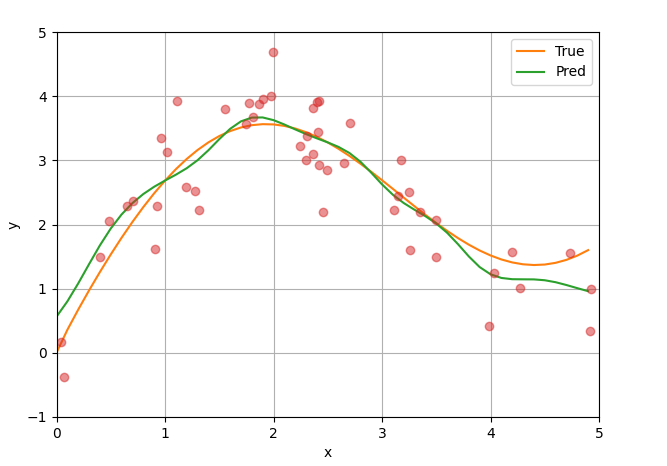
def plot_kernel_reg(y_hat):
    plt.plot(x_test,y_true,label='True')
    plt.plot(x_test, y_hat,label='Pred')
    plt.plot(x_train,y_train,'o',alpha=0.5)
    plt.legend()
    plt.xlim([0,5])
    plt.ylim([-1,5])
    plt.xlabel('x')
    plt.ylabel('y')
    plt.show()

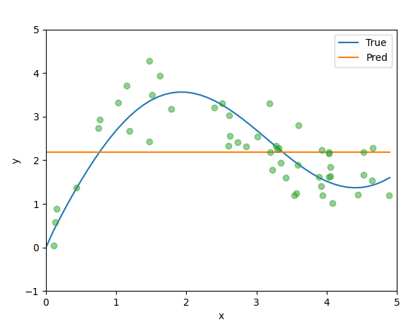
1.平均汇聚

#平均：基于平均汇聚来计算所有训练样本输出值的平均值
y_hat=torch.repeat_interleave(y_train.mean(),n_test)
plot_kernel_reg(y_hat)

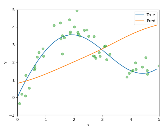
2.非参数注意力汇聚

按照距离远近给予权重，如果距离近，则给予较大权重

x_repeat=x_test.repeat_interleave(n_train).reshape(-1,n_train)#形状改为(n_test，n_train)
attention_weights=nn.functional.softmax(-(x_repeat-x_train)**2/2,dim=1)#距离小，全重大，有-号
y_hat=torch.matmul(attention_weights,x_train)
plot_kernel_reg(y_hat)

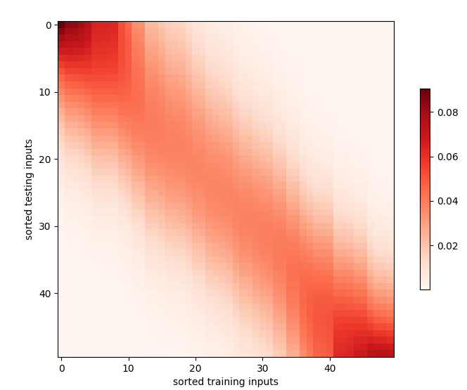
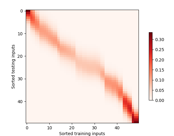
def show_heatmaps(matrices, xlabel, ylabel, titles=None, figsize=(2.5, 2.5), cmap='Reds'):

    # 获取矩阵的维度信息 (行数, 列数, Q的数量, K的数量)
    num_rows, num_cols,_,_= matrices.shape
    # 创建 matplotlib 的子图画布
    fig, axes = plt.subplots(num_rows, num_cols, figsize=figsize,
                             sharex=True, sharey=True, squeeze=False)
    # 遍历行和列，绘制每一个热力图
    for i, (row_axes, row_matrices) in enumerate(zip(axes, matrices)):
        for j, (ax, matrix) in enumerate(zip(row_axes, row_matrices)):
            # 绘制热力图 (将 PyTorch tensor 转换为 numpy 数组)
            pcm = ax.imshow(matrix.detach().numpy(), cmap=cmap)

            # 只在最底层显示 x 轴标签
            if i == num_rows - 1:
                ax.set_xlabel(xlabel)
            # 只在最左侧显示 y 轴标签
            if j == 0:
                ax.set_ylabel(ylabel)
            # 设置标题
            if titles:
                ax.set_title(titles[j])

    # 在所有子图的右侧添加一个统一的颜色条 (Colorbar)
    fig.colorbar(pcm, ax=axes, shrink=0.6)
    plt.show()
attention_weights_4d = attention_weights.unsqueeze(0).unsqueeze(0)
show_heatmaps(attention_weights_4d ,xlabel='sorted training inputs',ylabel='sorted testing inputs')

3.带参数注意力汇聚

class NWKernelRegression(nn.Module):
    def __init__(self, **kwargs):
        super().__init__(**kwargs)
        self.w=nn.Parameter(torch.randn(1,),requires_grad=True)
    def forward(self,queries,keys,values):
        queries=queries.repeat_interleave(keys.shape[1]).reshape((-1,keys.shape[1]))
        self.attention_weights=nn.functional.softmax(-((queries-keys)*self.w)**2/2,dim=1)
        return torch.bmm(self.attention_weights.unsqueeze(1),values.unsqueeze(-1)).reshape(-1)
x_tile=x_train.repeat((n_train,1))#重复n_train次，方便去除自己
y_tile=y_train.repeat((n_train,1))
keys=x_tile[(1-torch.eye(n_train)).type(torch.bool)].reshape((n_train,-1))#生成对角矩阵，然后在用1-，在转成布尔，过滤掉为0，即对角位置上的数，重新改形状
valus=y_tile[(1-torch.eye(n_train)).type(torch.bool)].reshape((n_train,-1))
net=NWKernelRegression()
loss=nn.MSELoss(reduction='none')
trainer=torch.optim.SGD(net.parameters(),lr=0.1)
animator=d2l.Animator(xlabel='epoch',ylabel='loss',xlim=[1,5])
for epoch in range(5):
    trainer.zero_grad()
    l=loss(net(x_train,keys,valus),y_train)
    l.sum().backward()
    trainer.step()
    print(f'epoch {epoch+1},loss {l.sum():.6f}')
    animator.add(epoch+1,float(l.sum()))
keys = x_train.repeat((n_test, 1))
# value的形状:(n_test，n_train)
values = y_train.repeat((n_test, 1))
y_hat = net(x_test, keys, values).unsqueeze(1).detach()
plot_kernel_reg(y_hat)
show_heatmaps(net.attention_weights.unsqueeze(0).unsqueeze(0),
                  xlabel='Sorted training inputs',
                  ylabel='Sorted testing inputs')