[TNNLS 2024]An Efficient Graph Learning System for Emotion Recognition Inspired by the Cognitive Pri

②For achieving effective EEG decoding and emotion recognition, they proposed Graph Convolutional Network framework with Brain network initial inspiration and Fused attention mechanism (BF-GCN)

③Datasets: SEED and SEED-IV

2.2. Introduction

①Non physiological signals such as posture, movement, and expression may conceal true emotions

2.3. Related Work

2.3.1. EEG-Based Emotion Recognition System

①2 widely used emotional models for affective computing: the discrete emotion model and the dimensional emotion model

②Introduced how other reseachers extract EEG features

2.3.2. Emotion Recognition With Deep Learning

①Lists some DL applied in emotion recognition

2.3.3. Transfer Learning of Emotion Recognition

②Domain generalization helps cross subject experiment

2.4. Methodology

①Overall framework:

2.4.1. Basic Theory of Spectral Graph Filtering

①A basic graph: $G=\{V,E,A\}$

②Laplacian matrix: $L=D-A$ where $D$ denotes degree matrix and $A$ denotes adjacency matrix

③Spectral graph filtering transform given spatial signal $x$ to $\widetilde{x}=U^Tx$ , where $U^T$ is graph filter obtained by $L=U\Lambda U^T$ , $U=[u_0,u_1,\ldots,u_{N-1}]$ is orthonormal Fourier basis of graph $G$ , $\Lambda=\operatorname{diag}([\lambda_0,\lambda_1,\ldots,\lambda_{N-1}])$

④Inverse graph Fourier transform:

$x=U\widetilde{x}=UU^Tx$

⑤Graph convolution in 2 signals in graph spectral domain:

$x_1*x_2=U\left(\left(U^Tx_1\right)\odot\left(U^Tx_2\right)\right)$

where $\odot$ denotes element wise Hadamard product

⑥A filtering function $g\left ( \cdot \right )$ can be applied as:

$y=g(L)x=g\left(U\Lambda U^T\right)x=Ug(\Lambda)U^Tx$

and further:

$y=g(L)x=Ug(\Lambda)U^Tx= \begin{bmatrix} Ug(\Lambda)\odot\left(U^Tx\right) \end{bmatrix} \\ =U\left\{\left[U^TUg(\Lambda)\right]\right\}\odot\left(U^Tx\right)=x*\left[Ug(\Lambda)\right].$

which can extract differential entropy (DE) feature in emotion EEG signals

2.4.2. BF-GCN Graph Learning System for Emotional EEG

（1）Processing and DE Feature Extraction of Emotional EEG

①Segmenting original signal to segments with a length of 1 s, and employing bandpass filtering including delta (1–4 Hz), theta (4–8 Hz), alpha (8–14 Hz), beta (14–30 Hz), and gamma (30–48 Hz)

②For EEG signals which are assumed to obey the Gaussian distribution have such a DE:

$\begin{aligned} \mathrm{DE}(X)= & -\int_{-\infty}^\infty\frac{1}{\sqrt{2\pi\sigma^2}}\exp\frac{(x-\mu)^2}{2\sigma^2}\log\frac{1}{\sqrt{2\pi\sigma^2}} \\ & \times\exp\frac{(x-\mu)^2}{2\sigma^2}dx=\frac{1}{2}\log(2\pi e\sigma^2) \end{aligned}$

where $X\sim N(\mu,\sigma^2)$ , $f(x)=(1/(2\pi\sigma^2)^{1/2})\exp-((x-\mu)^2/2\sigma^2)$

（2）Cognition-Inspired Functional Graph Branch

①Phase synchronization:

$\mathcal{P}_{xy}=\left|\frac{1}{T}\sum_1^Te^{i\Delta\varphi(t)}\right|,\quad\Delta\varphi(t)=\varphi_{X_x}(t)-\varphi_{X_y}(t)$

where $\mathcal{P}_{xy} \in [0,1]$ constructs adjacency matrix $A_c$

②The graph convolution operator of cognition-inspired functional graph branch:

$y_c=g(L_c)x=g\left(U_c\Lambda_cU_c^T\right)x=U_cg(\Lambda_c)U_c^Tx$

③Simplify feature extraction by $K$ -order Chebyshev polynomials:

$g(\Lambda_c)=\sum_{k=0}^{K-1}\theta_kT_k(\widetilde{\Lambda}_c)$

where $\theta_k$ is Chebyshev coefficient and $T_k\left ( x \right )$ is Chebyshec polynomial:

$\begin{cases} T_0(x)=1,T(x)_1=x \\ T_k(x)=2xT_{k-1}(x)-T_{k-2}(x) & \end{cases}$

④Graph convolution operator:

$\begin{aligned} \mathbf{y}_{c} & =U_cg(\Lambda_c){U_c}^Tx \\ & =\sum_{k=0}^{K-1}U_c \begin{bmatrix} \theta_kT_k\left(\widetilde{\lambda}_{c,0}\right) & \cdots & 0 \\ \vdots & \ddots & \vdots \\ 0 & \cdots & \theta_kT_k\left(\widetilde{\lambda}_{c,N-1}\right) \end{bmatrix}U_c^Tx \\ & =\sum_{k=0}^{K-1}\theta_kT_k(\widetilde{L}_c)x \end{aligned}$

where $\widetilde{L}_c=2L_c/\lambda_{c,\max}-I_N$ is scaled Laplacian, $\lambda_{c,\max}$ is the largest element among $\Lambda_{c}$ . They defined $\lambda_{c,\max}=2$

⑤The output of the cognition-inspired functional graph branch:

$Z_c=\mathrm{Relu}\left(\sum_{k=0}^{K-1}\theta_kT_k(\widetilde{L}_c)x\right)$

（3）Data-Driven Graph Branch

①Loss: they combined cross entropy ( $C_e$ ) and backpropagation (BP) algorithm:

$\mathrm{Loss}=C_e(l,l^p)+\alpha\|\Theta\|$

where $l$ denotes ground truth and $l^p$ is predicted label, $\Theta$ denotes model parameters and $\alpha$ is hyper parameter

②Updating adjacency matrix by:

$A_d=(1-\rho)A_d+\rho\frac{\partial\mathrm{Loss}}{\partial A_d}$

③Graph convolution operator:

$Z_d=\mathrm{Relu}\left(\sum_{k=0}^{K-1}\theta_kT_k(\widetilde{L}_d)x\right)$

（4）Fused Common Graph Branch

①2 spectral graph filter:

$\begin{gathered} Z_{fc}=\mathrm{Relu}\left(\sum_{k=0}^{K-1}\theta_kT_k(\widetilde{L}_c)x\right) \\ Z_{fd}=\mathrm{Relu}\left(\sum_{k=0}^{K-1}\theta_kT_k(\widetilde{L}_d)x\right) \end{gathered}$

②Loss for each branch:

$L_f=\|S_c-S_d\|_F^2$

where $S_c$ and $S_d$ are normalized embedding matrix, $S=Z_{\mathrm{nor}}\cdot Z_{\mathrm{nor}}^T$

（5）Attention Mechanism

①Applying attention on 3 spectral graph pattern:

$\begin{pmatrix} \omega_c,\omega_d,\omega_f \end{pmatrix}=\mathrm{Att} \begin{pmatrix} Z_c,Z_d,Z_f \end{pmatrix}$

where $\omega_c,\omega_d,\omega_f\quad\in\quad R^{n\times1}$ denotes attention values

②Attention function:

$\omega_c^i=q^T\cdot\tanh\left(W\cdot\left(z_c^i\right)^T+b\right)$

where 3 branches share the same weight matrix $W$

③Attention value for $Z_c$ on node $i$ :

$a_c^i=\mathrm{soft}\max\left(\omega_c^i\right)=\frac{\exp\left(\omega_c^i\right)}{\exp\left(\omega_c^i\right)+\exp\left(\omega_d^i\right)+\exp\left(\omega_f^i\right)}$

similar to other 2

④Final combined embedding:

$Z=\omega_c\cdot Z_c+\omega_d\cdot Z_d+\omega_f\cdot Z_f$

（6）Emotion Decoding Procedure

①Reducing the graph feature distribution difference between the source domain (training set) and the target domain (testing set) by graph domain adversarial:

$p_j\left(0|X_i^S,\theta_D\right)=\mathrm{softmax}_0\left(N_D\left(Z_{ij}^S\right)\right)\\p_j\left(1|X_i^T,\theta_D\right)=\mathrm{softmax}_1\left(N_D\left(Z_{ij}^T\right)\right)$

where $N_D$ is a two layer fully connected neural network. 0 is source label and 1 denotes target domain

②Optimal domain classifier:

$L_D=-\sum_i\left(\log(p(0|X_i^S,\theta_D))+\log(p(1|X_i^T,\theta_D))\right)$

③Total loss by adding gradient reversal layer (GRL) $\beta=(2/1+e^{-10p})-1$ and $p \in [0,1]$ :

$L=\mathrm{Loss}+\beta L_D+\gamma L_f$

where $\gamma$ is conformance constraint parameter

2.5. Experiments and Results

①Datasets: SEED, SEED IV

②EEG electrodes: 64 channels

③Bandpass filter: delta 1–4 Hz, theta 4–8 Hz, alpha 8–14 Hz, beta 14–30 Hz, and gamma 30–48 Hz

④Layer of graph conv: 2

⑤Dropout rate: 0.5

⑥Optimizer: Adam with 0.005 learning rate in subject-dependent experiments and 0.008 in subject-independent experiments

⑦Max epoch: 400

⑧Batch size: 64

⑨L2 regularization is in [1e-3, 3e-2]

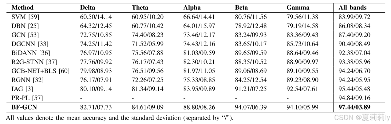
2.5.1. Subject-Dependent Experiments

①Data split: first 9 trials of EEG signals for training and remaining 6 for testing

②Performance on 5 bands on SEED:

③4 categories classification on SEED IV:

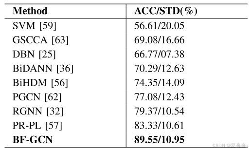
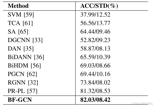
2.5.2. Subject-Independent Experiments

①They applied leaveone-subject-out cross-validation (LOSOCV) of 15 subjects on subject-independent experiments, on SEED:

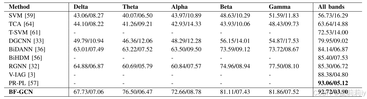
and on SEED IV:

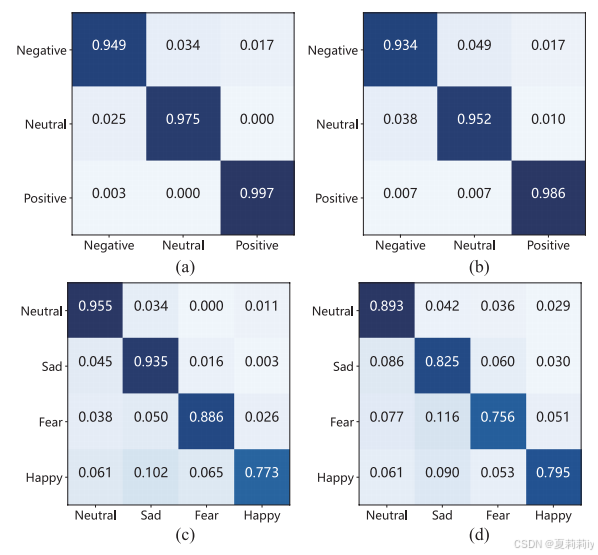
2.5.3. Confusion Matrix on Two Datasets

①Confusion matrices on SEED:

2.6. Analysis and Discussion

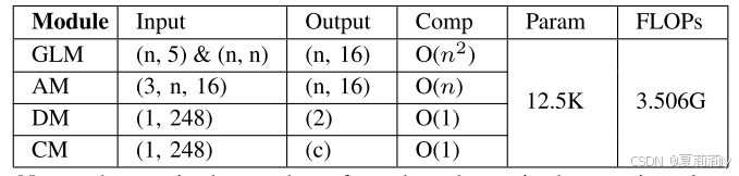
2.6.1. Computational Efficiency Analysis

①Parameters calculated by Torch-OpCounter (THOP) toolbox

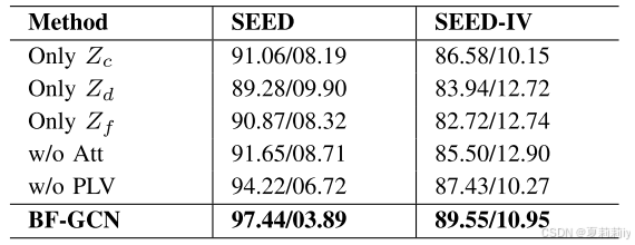
2.6.2. Ablation Study

①Feature and module ablation:

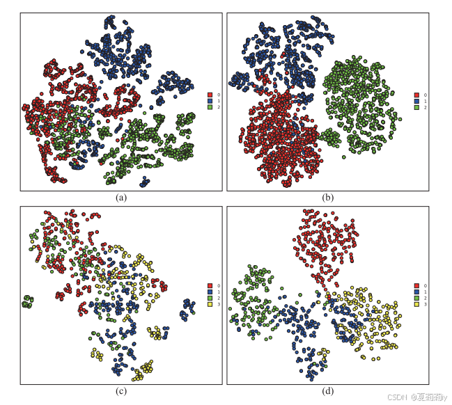
2.6.3. Visualization Analysis

①t-SNE visualization on SEED (the first row) and SEED IV (the second row):

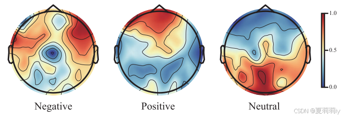
2.6.4. Cognitive Graph Pattern Analysis

①Brain activation mapping:

2.7. Conclusion

3. 知识补充

3.1. Phase Locking Value

（1）参考学习：PLV（Phase Locking Value，相位锁定值）的原理和计算-CSDN博客

3.2. logarithm energy spectrum

EEG（脑电图）的 对数能量谱（Logarithm Energy Spectrum） 是一种将 EEG 信号的频域能量分布进行对数变换后的表示方式，主要用于分析信号在不同频率上的能量强度，同时压缩动态范围以增强特征的可解释性

4. Reference

@article{li2024efficient,
  title={An Efficient Graph Learning System for Emotion Recognition Inspired by the Cognitive Prior Graph of EEG Brain Network},
  author={Li, Cunbo and Tang, Tian and Pan, Yue and Yang, Lei and Zhang, Shuhan and Chen, Zhaojin and Li, Peiyang and Gao, Dongrui and Chen, Huafu and Li, Fali and others},
  journal={IEEE Transactions on Neural Networks and Learning Systems},
  year={2024},
  publisher={IEEE}
}

脑启社区

脑启社区是一个专注类脑智能领域的开发者社区。欢迎加入社区，共建类脑智能生态。社区为开发者提供了丰富的开源类脑工具软件、类脑算法模型及数据集、类脑知识库、类脑技术培训课程以及类脑应用案例等资源。

更多推荐

YOLOv11【第四章：巅峰前沿与融合篇·第13节】生物计算与神经形态硬件：Spike 脉冲神经网络替换 YOLOv11！

脑启社区

EM-Core 创造者叙事：从牛角尖，到通用智能架构

脑启社区

加密货币开发者的终极天堂：探索ideas-for-projects-people-would-use中的$400奖金项目 [特殊字符]

你是否正在寻找创新的加密货币开发项目？ideas-for-projects-people-would-use项目为你提供了完美的解决方案！这个独特的开源项目汇集了众多实用的软件创意，其中加密货币领域的$400奖金项目更是开发者们的宝藏。本文将为你详细介绍这个项目的核心价值，帮助你快速找到适合自己的开发机会。## 🔍 项目概览与核心功能ideas-for-projects-people-w