神经网络部分重要操作
神经网络部分操作
神经网络部分重要操作
目录
0. 写在前面
1. 最大池化的使用
2. 非线性激活
3. 线性层及其他层介绍
4. 后记
0. 写在前面
关于神经网络的基本操作比较的多,这里只是简要介绍一些比较常见和重要的相关操作进行讲解。
1. 最大池化的使用
池化层在PyTorch中有很多,如图: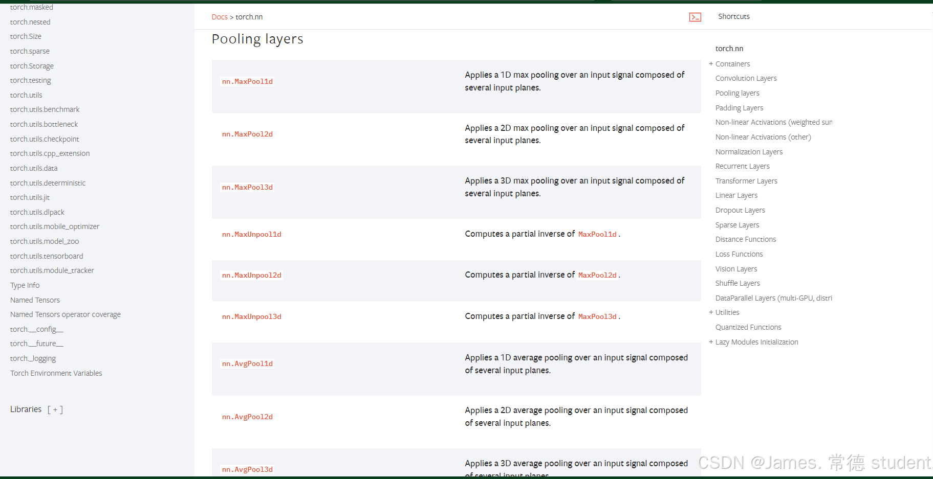
分为上采样,下采样,平均池化,自适应的最大池化。这里介绍最常用的最大池化: MaxPool2d
这是参数构成:
class torch.nn.MaxPool2d(kernel_size, stride=None, padding=0, dilation=1, return_indices=False, ceil_mode=False)
在输入信号(由多个输入平面组成)上应用2D最大池化操作。
在最简单的情况下,具有输入大小 ( N , C , H i n , W i n ) (N, C, H_{in}, W_{in}) (N,C,Hin,Win)的层输出大小为 ( N , C , H o u t , W o u t ) (N, C, H_{out}, W_{out}) (N,C,Hout,Wout),且核大小为 ( k H , k W ) (kH, kW) (kH,kW)的操作可以精确描述如下:
o u t p u t ( N i , C j , h , w ) = max m = 0 , . . . , k H − 1 max n = 0 , . . . , k W − 1 i n p u t ( N i , C j , s t r i d e [ 0 ] × h + m , s t r i d e [ 1 ] × w + n ) output(N_i, C_j, h, w) = \max_{m=0,...,kH-1} \max_{n=0,...,kW-1} input(N_i, C_j, stride[0] \times h + m, stride[1] \times w + n) output(Ni,Cj,h,w)=maxm=0,...,kH−1maxn=0,...,kW−1input(Ni,Cj,stride[0]×h+m,stride[1]×w+n)
如果填充不为零,则输入在两边都隐式地用负无穷大填充指定点数。膨胀控制着核点之间的间距。虽然难以描述,但这个链接有一个很好的可视化解释了膨胀的作用。
注意:
当ceil_mode=True时,滑动窗口允许超出边界,只要它们从左填充或输入开始的位置出发。从右填充区域开始的滑动窗口将被忽略。
参数kernel_size, stride, padding, dilation可以是:
- 一个单独的整数 – 在这种情况下,高度和宽度维度使用相同的值
- 两个整数的元组 – 在这种情况下,第一个整数用于高度维度,第二个整数用于宽度维度
参数
kernel_size (Union[int, Tuple[int, int]])- 窗口的最大值计算尺寸stride (Union[int, Tuple[int, int]])- 窗口的步长。默认值是kernel_sizepadding (Union[int, Tuple[int, int]])- 输入两侧隐式添加的负无穷大填充dilation (Union[int, Tuple[int, int]])- 控制窗口元素间步幅的参数return_indices (bool)- 如果为True,则返回最大值的索引以及输出。对后续的torch.nn.MaxUnpool2d有用ceil_mode (bool)- 当为True时,将使用ceil而不是floor来计算输出形状
形状
- 输入: ( N , C , H i n , W i n ) (N, C, H_{in}, W_{in}) (N,C,Hin,Win) 或 ( C , H i n , W i n ) (C, H_{in}, W_{in}) (C,Hin,Win)
- 输出: ( N , C , H o u t , W o u t ) (N, C, H_{out}, W_{out}) (N,C,Hout,Wout) 或 ( C , H o u t , W o u t ) (C, H_{out}, W_{out}) (C,Hout,Wout),其中
H o u t = ⌊ H i n + 2 × p a d d i n g [ 0 ] − d i l a t i o n [ 0 ] × ( k e r n e l _ s i z e [ 0 ] − 1 ) − 1 s t r i d e [ 0 ] + 1 ⌋ H_{out} = \left\lfloor\frac{H_{in} + 2 \times padding[0] - dilation[0] \times (kernel\_size[0] - 1) - 1}{stride[0]} + 1\right\rfloor Hout=⌊stride[0]Hin+2×padding[0]−dilation[0]×(kernel_size[0]−1)−1+1⌋
W o u t = ⌊ W i n + 2 × p a d d i n g [ 1 ] − d i l a t i o n [ 1 ] × ( k e r n e l _ s i z e [ 1 ] − 1 ) − 1 s t r i d e [ 1 ] + 1 ⌋ W_{out} = \left\lfloor\frac{W_{in} + 2 \times padding[1] - dilation[1] \times (kernel\_size[1] - 1) - 1}{stride[1]} + 1\right\rfloor Wout=⌊stride[1]Win+2×padding[1]−dilation[1]×(kernel_size[1]−1)−1+1⌋
其中ceil_mode=True,我们需要对不完全的数字进行保留,具体如图: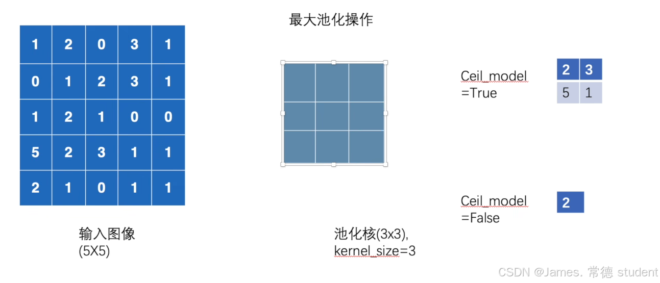
下面我们编写代码实现这一功能:
import torch
from torch.nn import MaxPool2d
from torch import nn
input_ = torch.tensor([[1, 2, 0, 3, 1],
[0, 1, 2, 3, 1],
[1, 2, 1, 0, 0],
[5, 2, 3, 1, 1],
[2, 1, 0, 1, 1]], dtype=torch.float32)
input_ = torch.reshape(input_, (-1, 1, 5, 5))
class James(nn.Module):
def __init__(self):
super(James, self).__init__()
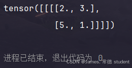
self.maxpool1 = MaxPool2d(3, ceil_mode=True)
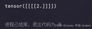
# self.maxpool2 = MaxPool2d(3, ceil_mode=False)
def forward(self, x):
output = self.maxpool1(x)
return output
james = James()
output = james(input_)
print(output)
结果如下:
一句话说明一下最大池化的作用:保留输入的特征同时将数据量减小。
下面我们依旧还是使用我们之前下载的FashionMNIST数据集进行操作:
import torch
import torchvision

from torchvision import transforms
from torch.utils.data import DataLoader
from torch.nn import MaxPool2d
from torch import nn
from torch.utils.tensorboard import SummaryWriter

class James(nn.Module):
    def __init__(self):
        super(James, self).__init__()
        self.maxpool1 = MaxPool2d(3, ceil_mode=True)
        self.maxpool2 = MaxPool2d(3, ceil_mode=False)

    def forward(self, x):
        output = self.maxpool1(x)
        return output

trans_pool = transforms.Compose([
    transforms.ToTensor(),
])

dataset_pool = torchvision.datasets.FashionMNIST("./data", train=False, transform=trans_pool, download=True)
dataloader = DataLoader(dataset=dataset_pool, batch_size=64)


def run_maxpool():
    james = James()
    writer = SummaryWriter("logs")
    step = 0

    for data in dataloader:
        imgs, targets = data
        writer.add_images("maxpool_input", imgs, step)
        output = james(imgs)
        writer.add_images("maxpool_output", output, step)
        step = step + 1

    writer.close()


if __name__ == "__main__":
    run_maxpool()
得到的结果如下: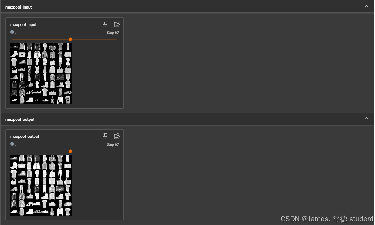
我们可以发现,图像变得模糊了,但是还是最大程度的保留了输入图像的信息。这样的好处就是在训练神经网络的时候训练量就会大大的减小,进而可以加快神经网络的训练。
2. 非线性激活
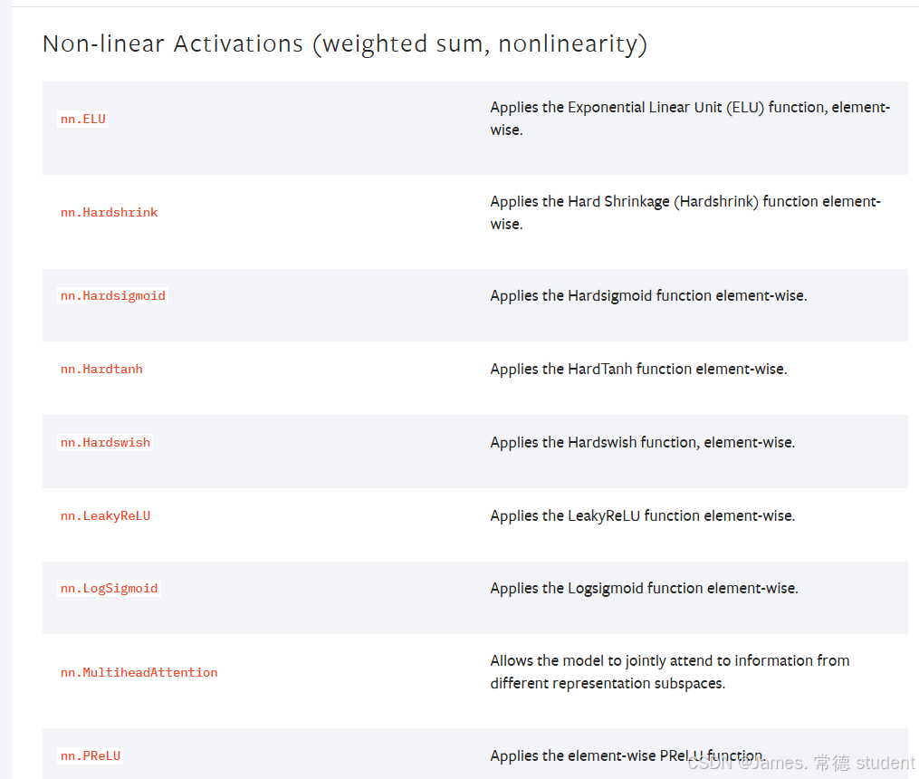
非线性激活的主要目的就是向神经网络当中引入一些非线性的特质。最常见的有ReLU、sigmoid、tanh。
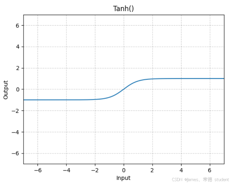
官方文档中对于ReLU和Sigmoid激活函数的输入有如下定义:
-
Input: ( ∗ ) (*) (∗), where
*means any number of dimensions. -
Output: ( ∗ ) (*) (∗), same shape as the input.
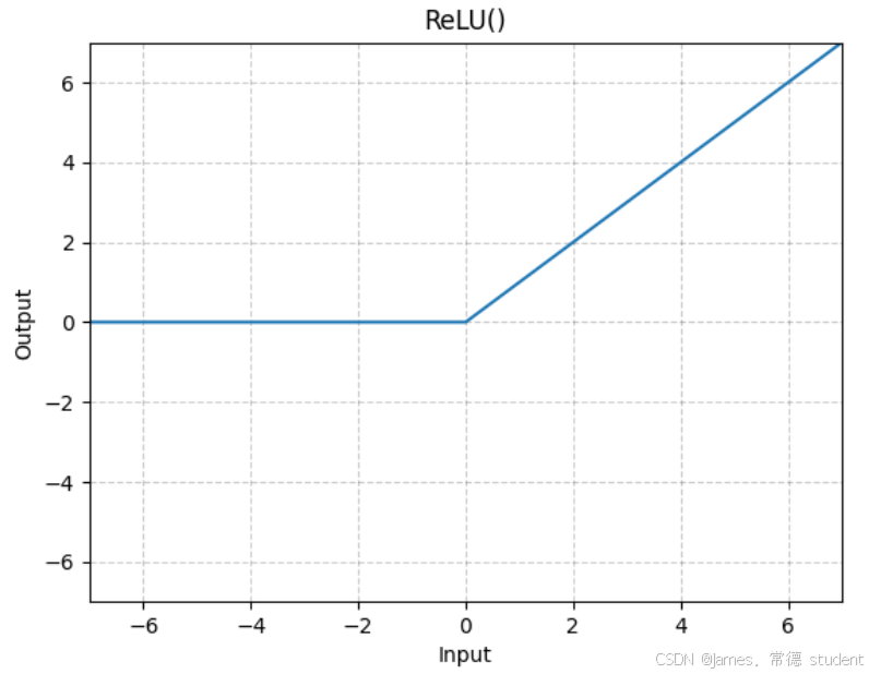
下面给一个简单的示例展示ReLU的作用:
import torch
from torch import nn
from torch.nn import ReLU

class James(nn.Module):
    def __init__(self):
        super(James, self).__init__()
        self.relu1 = ReLU()
        # 这里的 inplace 表示在不在原来的位置进行替换,True 表示在原来的位置进行替换,一般使用默认的False

    def forward(self, input):
        output = self.relu1(input)
        return output

def run():
    input = torch.tensor([[1, -0.5],
                          [-1, 3]])
    # input = torch.reshape(input, (-1, 1, 2, 2))  # 新版的不需要,老版的需要指定 batchsize
    # print(input.shape)
    james = James()
    output = james(input)
    print(output)

if __name__ == "__main__":
    run()
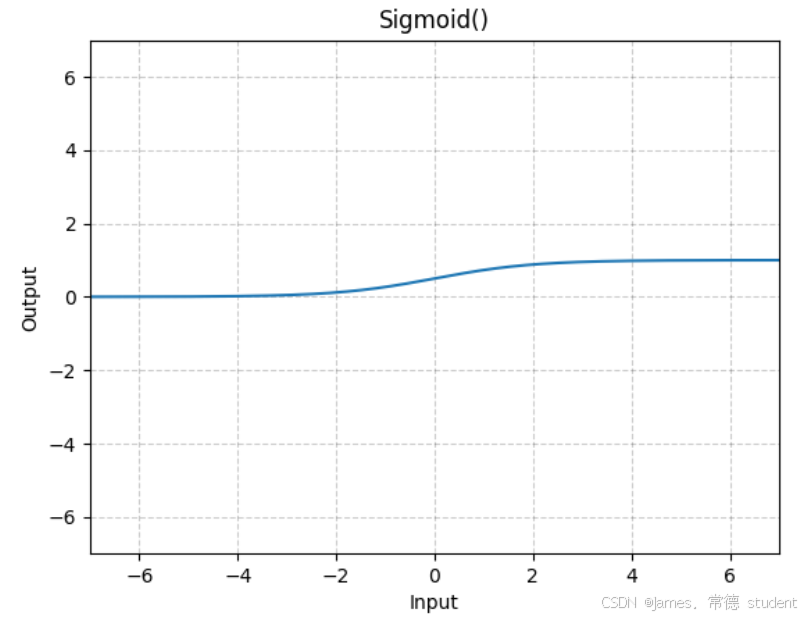
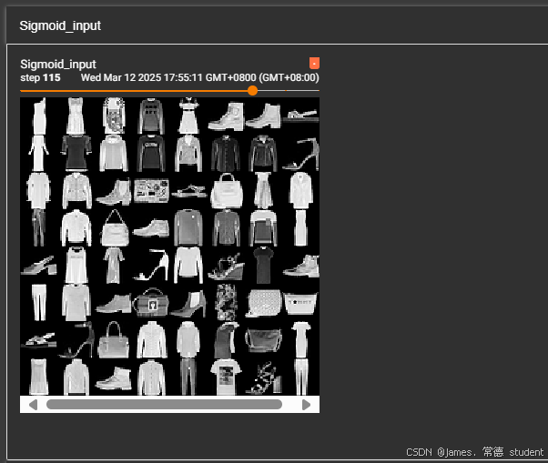
那么激活函数如何作用在数据集中呢,这里由于ReLU函数对图像的处理不是很明显,因此我们换成SIgmoid函数进行图像的处理,具体的代码如下:
import torch
import torchvision
from torch import nn
from torch.nn import ReLU, Sigmoid
from torch.utils.data import DataLoader
from torch.utils.tensorboard import SummaryWriter
class James(nn.Module):
def __init__(self):
super(James, self).__init__()
self.relu1 = ReLU()
self.sigmoid1 = Sigmoid()
def forward(self, input):
output = self.sigmoid1(input)
return output
def sigmoid_run():
dataset = torchvision.datasets.FashionMNIST("./data", train=False, download=True,
transform=torchvision.transforms.ToTensor())
dataloader = DataLoader(dataset, batch_size=64)
james = James()
writer = SummaryWriter("logs")
step = 0
for data in dataloader:
imgs, targets = data
writer.add_images("Sigmoid_input", imgs, step)
output = james(imgs)
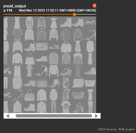
writer.add_images("sigmoid_output", output, step)
step += 1
writer.close()
if __name__ == "__main__":
sigmoid_run()
输出的结果为:
3. 线性层及其他层介绍
首先给出LINEAR 的相关定义和所需参数的具体含义:
Linear
class torch.nn.Linear(in_features, out_features, bias=True, device=None, dtype=None)[source]
对输入数据应用仿射线性变换:
$ y = xA^T + b $
该模块支持 TensorFloat32。
在某些 ROCm 设备上,当使用 float16 输入时,此模块会在反向传播中使用不同的精度。
参数
-
in_features (int)– 每个输入样本的大小 -
out_features (int)– 每个输出样本的大小 -
bias (bool)– 如果设置为 False,则该层不会学习加法偏置。默认值为 True
形状
-
输入: ( ∗ , H i n ) (*, H_{in}) (∗,Hin) 其中
*表示任意数量的维度(包括零维),且 H i n = i n _ f e a t u r e s H_{in} = in\_features Hin=in_features -
输出: ( ∗ , H o u t ) (*, H_{out}) (∗,Hout) 其中除最后一个维度外的所有维度都与输入具有相同的形状,且 H o u t = o u t _ f e a t u r e s H_{out} = out\_features Hout=out_features
变量
-
weight (torch.Tensor)– 模块的可学习权重,形状为 ( o u t _ f e a t u r e s , i n _ f e a t u r e s ) (out\_features, in\_features) (out_features,in_features)。其值从均匀分布 U ( − k , k ) U(-\sqrt{k}, \sqrt{k}) U(−k,k) 中初始化,其中 k = 1 i n _ f e a t u r e s k = \frac{1}{in\_features} k=in_features1 -
bias (torch.Tensor)– 模块的可学习偏置,形状为 ( o u t _ f e a t u r e s ) (out\_features) (out_features)。如果bias为 True,其值从均匀分布 U ( − k , k ) U(-\sqrt{k}, \sqrt{k}) U(−k,k) 中初始化,其中 k = 1 i n _ f e a t u r e s k = \frac{1}{in\_features} k=in_features1
线性层
class torch.nn.Linear(in_features, out_features, bias=True, device=None, dtype=None)[source]
对输入数据应用仿射线性变换:
y = x A T + b y = xA^T + b y=xAT+b
该模块支持 TensorFloat32。
在某些 ROCm 设备上,当使用 float16 输入时,此模块会在反向传播中使用不同的精度。
参数
-
in_features (int)– 每个输入样本的大小 -
out_features (int)– 每个输出样本的大小 -
bias (bool)– 如果设置为 False,则该层不会学习加法偏置。默认值为 True
形状
-
输入: ( ∗ , H i n ) (*, H_{in}) (∗,Hin) 其中
*表示任意数量的维度(包括零维),且 H i n = i n _ f e a t u r e s H_{in} = in\_features Hin=in_features -
输出: ( ∗ , H o u t ) (*, H_{out}) (∗,Hout) 其中除最后一个维度外的所有维度都与输入具有相同的形状,且 H o u t = o u t _ f e a t u r e s H_{out} = out\_features Hout=out_features
变量
-
weight (torch.Tensor)– 模块的可学习权重,形状为 ( o u t _ f e a t u r e s , i n _ f e a t u r e s ) (out\_features, in\_features) (out_features,in_features)。其值从均匀分布 U ( − k , k ) U(-\sqrt{k}, \sqrt{k}) U(−k,k) 中初始化,其中 k = 1 i n _ f e a t u r e s k = \frac{1}{in\_features} k=in_features1 -
bias (torch.Tensor)– 模块的可学习偏置,形状为 ( o u t _ f e a t u r e s ) (out\_features) (out_features)。如果bias为 True,其值从均匀分布 U ( − k , k ) U(-\sqrt{k}, \sqrt{k}) U(−k,k) 中初始化,其中 k = 1 i n _ f e a t u r e s k = \frac{1}{in\_features} k=in_features1
编写下列代码进行相关的练习:
import torchvision
import torch
from torch import nn

from torch.nn import Linear
from torch.utils.data import DataLoader

dataset_pool = torchvision.datasets.FashionMNIST("./data", train=False, transform=torchvision.transforms.ToTensor(),
                                                 download=True)

dataloader = DataLoader(dataset=dataset_pool, batch_size=64, drop_last=True)
# 这里需要丢弃掉最后一组,因为最后一组的图片没有64张


class James(nn.Module):
    def __init__(self):
        super(James, self).__init__()
        # 根据 FashionMNIST 图像的尺寸 (28x28) 和单通道,计算输入特征数
        self.linear1 = Linear(in_features=28 * 28 * 64, out_features=10)

    def forward(self, x):
        output = self.linear1(x)
        return output


def linear_run():
    james = James()
    for data in dataloader:
        imgs, targets = data
        print(imgs.shape)
        # output = torch.reshape(imgs, (1, 1, 1, -1))
        # reshape 功能强大,可以指定尺寸进行变换
        output = torch.flatten(imgs)
        # flatten 会将 tensor 变成一行
        print(output.shape)
        output = james(output)
        print(output.shape)


if __name__ == "__main__":
    linear_run()
4. 后记
上述只是列举了一些常见的操作,相关的原理并没有讲清楚,只是进一步认识了PyTorch框架。
到此,我们大致可以基于之前的内容搭建网络了,实际上,许多经典的架构如:AlexNet,GoogleNet,Transformer等已经在PyTorch中封装好了,需要用时可以自行调用。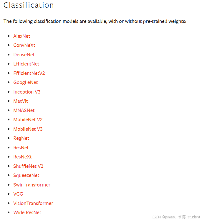
限于笔者的能力,上述文章肯定有众多不足之处,还请读者多多包涵,并提出宝贵的改进意见。
**正如宋代诗人黄庭坚的《跋子瞻和陶诗》中的诗句:
“文章千古事,得失寸心知。作者皆成今古,读者何必旧新。”

脑启社区是一个专注类脑智能领域的开发者社区。欢迎加入社区,共建类脑智能生态。社区为开发者提供了丰富的开源类脑工具软件、类脑算法模型及数据集、类脑知识库、类脑技术培训课程以及类脑应用案例等资源。
更多推荐


 20
20 0
0- 0


 已为社区贡献2条内容

所有评论(0)