【机器学习】逻辑回归

逻辑斯谛回归是一种用于二分类问题的广义线性模型，通过线性假设对样本标签进行建模。其基本形式为特征向量与待估计参数的线性组合，通过逻辑函数将输出映射到[0,1]区间，表示样本属于某一类的概率。模型训练通过最大似然估计优化参数，通常使用梯度下降法等优化算法。模型评估常用混淆矩阵、准确率、召回率、F1值、ROC曲线和AUC值等指标。逻辑斯谛回归具有较好的可解释性和可并行性，广泛应用于医学、营销学和金融学

2401_84149564

1571人浏览 · 2025-05-15 18:39:46

2401_84149564 · 2025-05-15 18:39:46 发布

一、逻辑斯谛回归概述

在线性回归中，我们利用了参数化的线性假设解决了回归问题，而分类问题作为机器学习任务中的另一大类别，其回归问题既有相似之处也有不同之处。通常来说，回归问题的输出是连续的，而分类问题的输出是离散的。在大多数时候我们可以只考虑最简单的二分类问题，样本标签

$y\epsilon \left \{ 0,1 \right \}$ ，利用线性假设对问题建模，这一模型就是逻辑斯谛回归（logistic regression），又称为对数几率回归。

二、逻辑斯谛回归模型

逻辑斯谛回归是一种用于二分类问题的广义线性模型，它的基本形式为：
$P(Y=1|X)=\frac{1}{1+e^{-(w_0+w_1x_1+w_2x_2+\cdots+w_nx_n)}}$
其中， $X=(x_1,x_2,\cdots,x_n)$ 是特征向量，Y是分类变量， $w_0,w_1,\cdots,w_n$ 是待估计的参数。
似然函数的构建
对于给定的训练数据集 $\{(x_i,y_i)\}_{i=1}^m$ ，其中 $x_i$ 是第i个样本的特征向量， $y_i$ 是第i个样本的分类标签 $(y_i\in\{0,1\})$ ，似然函数是在给定模型参数下，观察到这些数据的概率。由于样本之间相互独立，所以似然函数可以表示为各个样本概率的乘积：
$L(w)=\prod_{i=1}^m P(y_i|x_i;w)$
对于逻辑斯谛回归， $P(y_i|x_i;w)$ 可以根据模型的定义得到：
当 $y_i = 1$ 时， $P(y_i|x_i;w)=\frac{1}{1+e^{-(w_0+w_1x_{i1}+w_2x_{i2}+\cdots+w_nx_{in})}}$
当 $y_i = 0$ 时， $P(y_i|x_i;w)=1-\frac{1}{1+e^{-(w_0+w_1x_{i1}+w_2x_{i2}+\cdots+w_nx_{in})}}$
将其代入似然函数中，得到：
$L(w)=\prod_{i=1}^m [y_i\frac{1}{1+e^{-(w_0+w_1x_{i1}+w_2x_{i2}+\cdots+w_nx_{in})}}+(1-y_i)(1-\frac{1}{1+e^{-(w_0+w_1x_{i1}+w_2x_{i2}+\cdots+w_nx_{in})}})]$
对数似然函数
直接优化似然函数比较困难，因为似然函数中包含乘积项，求导后形式复杂。为了简化计算，通常对似然函数取对数，得到对数似然函数：
$\ell(w)=\log L(w)=\sum_{i=1}^m [y_i\log(\frac{1}{1+e^{-(w_0+w_1x_{i1}+w_2x_{i2}+\cdots+w_nx_{in})}})+(1-y_i)\log(1-\frac{1}{1+e^{-(w_0+w_1x_{i1}+w_2x_{i2}+\cdots+w_nx_{in})}})]$
最大似然估计
最大似然估计的目标是找到一组参数w，使得对数似然函数 $\ell(w)$ 最大。这是一个无约束的优化问题，可以使用多种优化算法来求解，如梯度下降法、牛顿法等。
以梯度下降法为例，首先计算对数似然函数对参数w_j的偏导数：
$\frac{\partial\ell(w)}{\partial w_j}=\sum_{i=1}^m [y_i\frac{x_{ij}e^{-(w_0+w_1x_{i1}+w_2x_{i2}+\cdots+w_nx_{in})}}{1+e^{-(w_0+w_1x_{i1}+w_2x_{i2}+\cdots+w_nx_{in})}}-(1-y_i)\frac{x_{ij}e^{w_0+w_1x_{i1}+w_2x_{i2}+\cdots+w_nx_{in}}}{1+e^{w_0+w_1x_{i1}+w_2x_{i2}+\cdots+w_nx_{in}}}]$
然后，根据梯度下降法的更新公式 $w_j=w_j-\alpha\frac{\partial\ell(w)}{\partial w_j}$ ，其中 $\alpha$ 是学习率，不断更新参数w，直到收敛。

三、模型评估

1.混淆矩阵：混淆矩阵是评估分类模型性能的常用工具，它展示了模型预测结果与真实标签之间的关系。对于二分类问题，混淆矩阵如下：

	正例	反例
正例	真正例	假反例
反例	假正例	真反例

其中，TP表示真正例（True Positive），即模型预测为正例且实际为正例的样本数量；FN表示假反例（False Negative），即模型预测为反例但实际为正例的样本数量；FP表示假正例（False Positive），即模型预测为正例但实际为反例的样本数量；TN表示真反例（True Negative），即模型预测为反例且实际为反例的样本数量。
1.准确率（Accuracy）：准确率是指模型预测正确的样本数量占总样本数量的比例，计算公式为：
   $Accuracy=\frac{TP+TN}{TP+FP+FN+TN}$
准确率可以直观地反映模型的整体性能，但在样本不平衡的情况下，准确率可能会受到影响。
2.召回率（Recall）：召回率是指模型预测为正例的样本中，实际为正例的样本数量占实际正例样本数量的比例，计算公式为：
   $Recall=\frac{TP}{TP+FN}$
召回率关注的是模型对正例的识别能力，在一些对正例敏感的应用场景中，如疾病检测等，召回率是一个重要的评估指标。
3.F1值（F1-score）：F1值是准确率和召回率的调和平均数，计算公式为：
   $F1=\frac{2\times Precision\times Recall}{Precision+Recall}$
其中， $Precision=\frac{TP}{TP+FP}$ 表示精确率。F1值综合考虑了准确率和召回率，能够更全面地评估模型的性能。
4.ROC曲线和AUC值：ROC曲线（Receiver Operating Characteristic Curve）是以假正率（False Positive Rate， $FPR=\frac{FP}{FP+TN}$ ）为横坐标，真正率（True Positive Rate， $TPR=\frac{TP}{TP+FN}$ ）为纵坐标绘制的曲线。AUC值（Area Under the Curve）是ROC曲线下的面积，取值范围在0到1之间。AUC值越大，说明模型的性能越好。
5.对数损失（Log Loss）：对数损失是一种基于概率的损失函数，用于衡量模型预测概率与真实标签之间的差异，计算公式为：
$LogLoss=-\frac{1}{m}\sum_{i=1}^m [y_i\log(p_i)+(1-y_i)\log(1-p_i)]$
其中，m是样本数量， $y_i$ 是第i个样本的真实标签， $p_i$ 是第i个样本预测为1的概率。对数损失越小，说明模型的性能越好。

四、Python实现逻辑斯谛回归

采用随机生成便于进行二分类的数据集，划分为训练集和预测集，训练集部分采用自定义的逻辑斯谛回归模型和使用sklearn库中的逻辑斯谛回归模型。自定义模型部分包括了梯度下降法训练模拟，计算损失，准确率等信息。可视化部分将自定义的和sklearn库中的逻辑斯谛回归模型在同一图中展示，这样可以直观地比较出两个模型的分类效果。

Python代码如下：

print('手动和sklearn库实现逻辑斯谛回归')
import numpy as np
import matplotlib.pyplot as plt
from matplotlib.ticker import MaxNLocator

# 随机生成2000个样本的数据集
np.random.seed(42)
num_samples = 2000

# 增大类别间距，减小方差
mean_class0 = [0, 0]       # 类别0均值
mean_class1 = [3, 3]       # 类别1均值
cov = [[0.5, 0], [0, 0.5]] # 协方差矩阵

# 生成样本数据
x_class0 = np.random.multivariate_normal(mean_class0, cov, num_samples // 2)
x_class1 = np.random.multivariate_normal(mean_class1, cov, num_samples // 2)
x_total = np.vstack((x_class0, x_class1))
y_total = np.hstack((np.zeros(num_samples // 2), np.ones(num_samples // 2)))

print('数据集大小：', len(x_total))

# 数据可视化
pos_index = np.where(y_total == 1)
neg_index = np.where(y_total == 0)
plt.scatter(x_total[pos_index, 0], x_total[pos_index, 1], marker='o', color='coral', s=10)
plt.scatter(x_total[neg_index, 0], x_total[neg_index, 1], marker='x', color='blue', s=10)
plt.xlim(-2, 5)
plt.ylim(-2, 5)
plt.xlabel('X1 axis')
plt.ylabel('X2 axis')
plt.title('Enhanced Separable Dataset')
plt.show()

# 划分训练集与测试集
np.random.seed(0)
ratio = 0.7
split = int(len(x_total) * ratio)
idx = np.random.permutation(len(x_total))
x_total = x_total[idx]
y_total = y_total[idx]
x_train_raw, y_train = x_total[:split], y_total[:split]
x_test_raw, y_test = x_total[split:], y_total[split:]

# 数据标准化（保持原始数据用于sklearn）
x_mean = x_train_raw.mean(axis=0)
x_std = x_train_raw.std(axis=0)
x_train = (x_train_raw - x_mean) / x_std
x_test = (x_test_raw - x_mean) / x_std
x_total = (x_total - x_mean) / x_std  # 用于最终可视化

# 为手动实现模型添加偏置项（创建新变量）
X_train = np.c_[np.ones(x_train.shape[0]), x_train]
X_test = np.c_[np.ones(x_test.shape[0]), x_test]
def acc(y_true, y_pred):
    return np.mean(y_true == y_pred)
def auc(y_true, y_pred):
    unique_classes = np.unique(y_true)
    if len(unique_classes) < 2:
        return 0.5
    idx = np.argsort(y_pred)[::-1]
    y_true = y_true[idx]
    tp = np.cumsum(y_true)
    fp = np.cumsum(1 - y_true)
    total_tp = tp[-1]
    total_fp = fp[-1]
    tpr = tp / total_tp if total_tp!= 0 else np.zeros_like(tp)
    fpr = fp / total_fp if total_fp!= 0 else np.zeros_like(fp)
    tpr = np.concatenate([[0], tpr])
    fpr = np.concatenate([[0], fpr])
    return np.trapz(tpr, fpr)
# 逻辑斯谛函数（数值稳定版）
def logistic(z):
    z = np.clip(z, -500, 500)  # 防止数值溢出
    return 1 / (1 + np.exp(-z))
def GD(num_steps, learning_rate, l2_coef):
    theta = np.random.normal(scale=0.1, size=(X_train.shape[1],))
    train_losses = []
    test_losses = []
    train_acc = []
    test_acc = []
    train_auc = []
    test_auc = []
    best_loss = float('inf')
    patience = 20
    no_improve = 0

    for i in range(num_steps):
        # 前向传播
        z = X_train @ theta
        pred = logistic(z)

        # 数值稳定处理
        epsilon = 1e-8
        pred = np.clip(pred, epsilon, 1 - epsilon)

        # 计算梯度
        grad = X_train.T @ (pred - y_train) + l2_coef * theta

        # 参数更新
        theta -= learning_rate * grad

        # 计算训练损失
        train_loss = (-y_train @ np.log(pred)
                      - (1 - y_train) @ np.log(1 - pred)
                      + 0.5 * l2_coef * theta @ theta) / len(y_train)
        train_losses.append(train_loss)

        # 计算测试集指标
        test_z = X_test @ theta
        test_pred = logistic(test_z)
        test_pred = np.clip(test_pred, epsilon, 1 - epsilon)
        test_loss = (-y_test @ np.log(test_pred)
                     - (1 - y_test) @ np.log(1 - test_pred)) / len(y_test)
        test_losses.append(test_loss)

        # 早停机制
        if train_loss < best_loss:
            best_loss = train_loss
            no_improve = 0
        else:
            no_improve += 1

        if no_improve >= patience:
            print(f'Early stopping at epoch {i}')
            break

        # 记录准确率和AUC
        train_acc.append(acc(y_train, pred >= 0.5))
        test_acc.append(acc(y_test, test_pred >= 0.5))
        train_auc.append(auc(y_train, pred))
        test_auc.append(auc(y_test, test_pred))

    return theta, train_losses, test_losses, train_acc, test_acc, train_auc, test_auc
# 超参数
num_steps = 300
learning_rate = 0.005
l2_coef = 0.1

theta, train_losses, test_losses, train_acc, test_acc, \
train_auc, test_auc = GD(num_steps, learning_rate, l2_coef)

# 绘图部分
plt.figure(figsize=(13, 9))
actual_steps = len(train_losses)
xticks = np.arange(actual_steps) + 1

plt.subplot(221)
plt.plot(xticks, train_losses, color='blue', label='train loss')
plt.plot(xticks, test_losses, color='red', ls='--', label='test loss')
plt.gca().xaxis.set_major_locator(MaxNLocator(integer=True))
plt.xlabel('Epochs')
plt.ylabel('Loss')
plt.legend()

plt.subplot(222)
plt.plot(xticks, train_acc, color='blue', label='train accuracy')
plt.plot(xticks, test_acc, color='red', ls='--', label='test accuracy')
plt.gca().xaxis.set_major_locator(MaxNLocator(integer=True))
plt.xlabel('Epochs')
plt.ylabel('Accuracy')
plt.legend()

plt.subplot(223)
plt.plot(xticks, train_auc, color='blue', label='train AUC')
plt.plot(xticks, test_auc, color='red', ls='--', label='test AUC')
plt.gca().xaxis.set_major_locator(MaxNLocator(integer=True))
plt.xlabel('Epochs')
plt.ylabel('AUC')
plt.legend()

# 在sklearn对比代码后添加以下可视化部分（替换原第4个子图）
# 提取sklearn模型参数
from sklearn.linear_model import LogisticRegression

lr_clf = LogisticRegression(
    penalty='l2',
    C=1 / (l2_coef * len(x_train)),
    solver='liblinear',
    fit_intercept=True  # 显式设置截距项
)
lr_clf.fit(x_train, y_train)  # 使用标准化后的原始数据（没有偏置项）
print('Sklearn准确率：', lr_clf.score(x_test, y_test))
print('Sklearn系数（含截距项）：', lr_clf.coef_[0], lr_clf.intercept_)

sk_theta = np.concatenate([lr_clf.intercept_, lr_clf.coef_.ravel()])

# 修改后的绘图代码（替换原plt.subplot(224)部分）
plt.subplot(224)
plot_x = np.linspace(-3, 4, 100)  # 根据标准化后数据调整范围

# 绘制手动模型的决策边界（蓝色虚线）
manual_boundary = -(theta[0] + theta[1] * plot_x) / theta[2]
plt.plot(plot_x, manual_boundary, ls='--', color='blue', label='Manual Model')

# 绘制sklearn的决策边界（红色实线）
sklearn_boundary = -(sk_theta[0] + sk_theta[1] * plot_x) / sk_theta[2]
plt.plot(plot_x, sklearn_boundary, ls='-', color='red', label='Sklearn Model')

# 数据点绘制
plt.scatter(x_total[pos_index, 0], x_total[pos_index, 1], marker='o', color='coral', s=10, alpha=0.6)
plt.scatter(x_total[neg_index, 0], x_total[neg_index, 1], marker='x', color='blue', s=10, alpha=0.6)

# 图形设置
plt.xlim(-3, 4)  # 根据标准化数据调整显示范围
plt.ylim(-3, 4)
plt.xlabel('Standardized X1')
plt.ylabel('Standardized X2')
plt.title('Decision Boundaries Comparison')
plt.legend()

plt.tight_layout()
plt.show()

# 测试结果
y_pred = np.where(logistic(X_test @ theta) >= 0.5, 1, 0)
final_acc = acc(y_test, y_pred)
print('预测准确率：', final_acc)
print('回归系数：', theta)

程序运行结果如下：

手动和sklearn库实现逻辑斯谛回归
数据集大小： 2000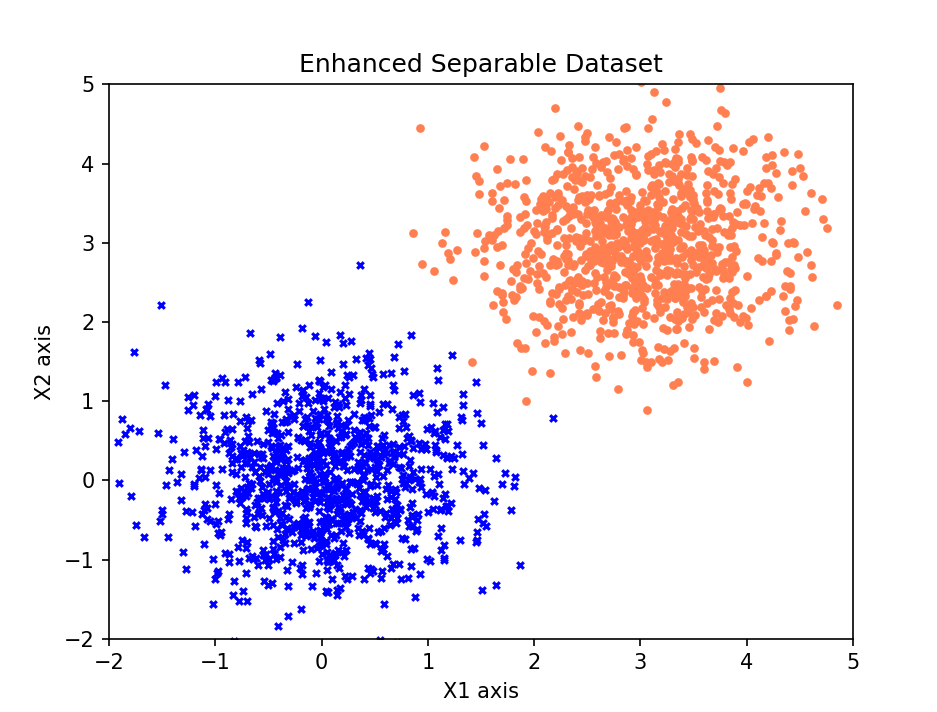

Sklearn准确率： 0.9983333333333333
Sklearn系数（含截距项）： [1.07314428 1.06127616] [0.00538514]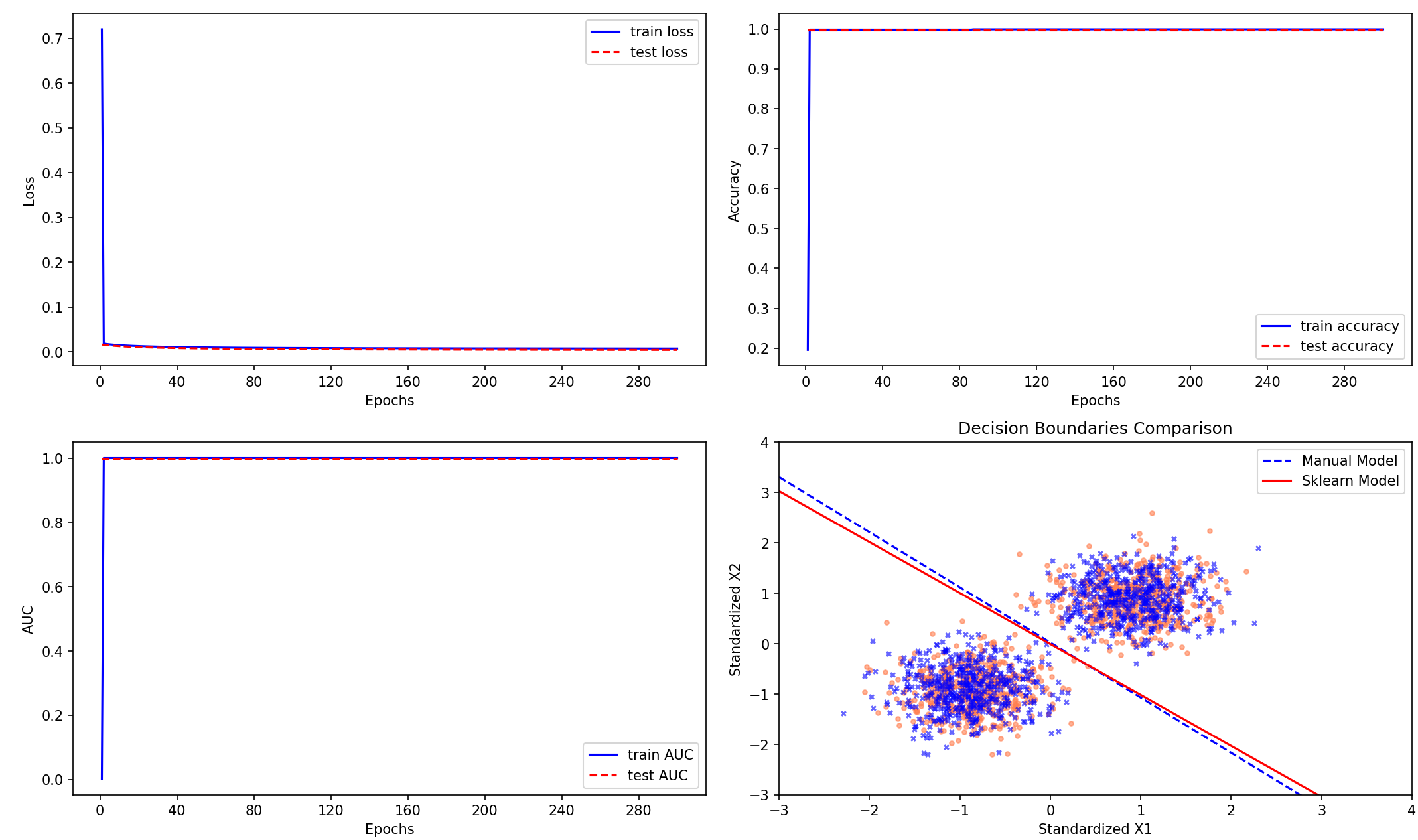

预测准确率： 0.9983333333333333
回归系数： [-0.13516334 5.96943086 5.45487076]

五、总结

逻辑斯谛回归是一种用于二分类问题的广义线性模型，通过线性假设对样本标签进行建模。其基本形式为特征向量与待估计参数的线性组合，通过逻辑函数将输出映射到[0,1]区间，表示样本属于某一类的概率。模型训练通过最大似然估计优化参数，通常使用梯度下降法等优化算法。模型评估常用混淆矩阵、准确率、召回率、F1值、ROC曲线和AUC值等指标。Python中可通过自定义实现或使用sklearn库进行逻辑斯谛回归模型的训练和评估。

逻辑斯谛回归，虽然其名字包含“回归”二字，但它是最具有代表性的机器学习分类模型，至今还在学习研究和工业落地场景中被广泛使用。逻辑斯谛回归具有较好的可解释性，其参数的绝对值大小和正负代表了对应的特征对于预测数据类别的重要性，在医学、营销学和金融学等领域广泛被用于目标归因。逻辑斯谛回归具有极好的可并行性，其优化目标相对参数是凸函数，具有全局唯一最优解，因此工业实践中也时常使用分布式并行训练的逻辑斯谛回归方法。