目录

 

1. 计算小批量的均值和方差

2. 标准化（Normalization）

3. 缩放与偏移（可学习参数）

4. 为什么要用 Batch Normalization？

5. 在训练和推理（测试）中的区别

6.深入理解BN

---

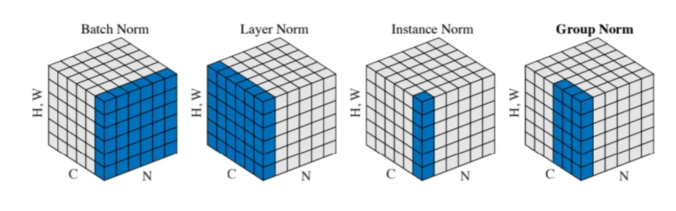
Batch Normalization（BN） 是一种加速深度神经网络训练并提高其稳定性的方法，由 Ioffe 和 Szegedy 在 2015 年提出。BN 的核心思想是对每一层的输入进行标准化，使其分布具有零均值和单位方差。

原理：

BN 是在每一个小批量（batch）中对激活值（或特征）进行归一化处理，主要包括以下几个步骤：

1. 计算小批量的均值和方差

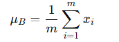
假设输入为一个小批量的激活值 x = [x₁, x₂, ..., xₘ]，其中 m 是 batch size，对每个维度进行如下计算：

均值（mean）：

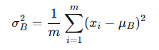
方差（variance）：

2. 标准化（Normalization）

将数据变为均值为 0、方差为 1：

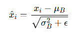
其中 ε 是一个很小的正数，防止除以 0。

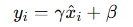
3. 缩放与偏移（可学习参数）

为了保留模型的表达能力，引入两个可学习参数：

• γ（scale）：缩放因子

• β（shift）：平移因子

最终输出：

4. 为什么要用 Batch Normalization？

主要优点：

1. 缓解内部协变量偏移（Internal Covariate Shift）：
   每一层输入分布更稳定，加快收敛速度。

2. 允许使用更高的学习率：
   降低了对权重初始化的敏感性。

3. 起到一定的正则化作用：
   减少对 Dropout 的依赖。

4. 训练更深的神经网络：
   有助于梯度更稳定地传播。

向量形式表示：

对于输入 X ∈ ℝ^{m×d}（m 是 batch size，d 是每个样本的维度）：

计算每个特征维度的均值和方差：

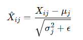
标准化：

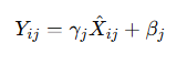
仿射变换：

5. 在训练和推理（测试）中的区别

• 训练时：使用当前 batch 的均值和方差。

• 推理时：使用训练过程中累计得到的滑动平均值（moving average）来替代 batch statistics。

6.深入理解BN

BN 的主要目标是：

缓解“内部协变量偏移（Internal Covariate Shift）”，即在训练过程中，每一层的输入分布随着前一层参数更新而发生变化，这使得训练变得困难、收敛变慢。

BN 主要解决了什么？

为了让每一层的输入保持在相对稳定、标准化的分布范围内（均值为0，方差为1），具有以下好处：

• 梯度更稳定，不会因为输入值过大或过小造成梯度爆炸或消失。

• 激活函数工作在非饱和区间（特别是 sigmoid / tanh），从而更有效地传播梯度。

• 提高网络收敛速度，常能使用更大学习率。

• 一定程度上抑制过拟合（类似正则化效果）。

7.pytorch实现BN代码

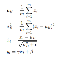
通过代码加深理解，再次回顾下公式（以 2D 数据为例）：

实现代码（简化版）

下面是一个 全连接层/特征维度 BN 的例子（适合全连接层或通道维度，卷积会在每个通道维度做 BN）：

import torch
import torch.nn as nn

class YOLOv1Full(nn.Module):
    def __init__(self, S=7, B=2, C=20):
        super(YOLOv1Full, self).__init__()
        self.S = S
        self.B = B
        self.C = C

        # 24 个卷积层
        self.features = nn.Sequential(
            # (3, 448, 448) -> (64, 224, 224)
            nn.Conv2d(3, 64, kernel_size=7, stride=2, padding=3),
            nn.LeakyReLU(0.1, inplace=True),
            nn.MaxPool2d(2, 2),

            # (64, 224, 224) -> (192, 112, 112)
            nn.Conv2d(64, 192, kernel_size=3, padding=1),
            nn.LeakyReLU(0.1, inplace=True),
            nn.MaxPool2d(2, 2),

            # (192, 112, 112) -> (128, 112, 112)
            nn.Conv2d(192, 128, kernel_size=1),
            nn.LeakyReLU(0.1, inplace=True),

            # (128, 112, 112) -> (256, 112, 112)
            nn.Conv2d(128, 256, kernel_size=3, padding=1),
            nn.LeakyReLU(0.1, inplace=True),

            # (256, 112, 112) -> (256, 112, 112)
            nn.Conv2d(256, 256, kernel_size=1),
            nn.LeakyReLU(0.1, inplace=True),

            # (256, 112, 112) -> (512, 112, 112)
            nn.Conv2d(256, 512, kernel_size=3, padding=1),
            nn.LeakyReLU(0.1, inplace=True),
            nn.MaxPool2d(2, 2),  # (512, 112, 112) -> (512, 56, 56)

            # 4 次重复的卷积块
            *self._make_conv_block(512, 256, 512),
            *self._make_conv_block(512, 256, 512),
            *self._make_conv_block(512, 256, 512),
            *self._make_conv_block(512, 512, 1024),

            nn.MaxPool2d(2, 2),  # (1024, 56, 56) -> (1024, 28, 28)

            # 2 次卷积块
            *self._make_conv_block(1024, 512, 1024),
            *self._make_conv_block(1024, 512, 1024),

            # 两次额外卷积
            nn.Conv2d(1024, 1024, kernel_size=3, padding=1),
            nn.LeakyReLU(0.1, inplace=True),
            nn.Conv2d(1024, 1024, kernel_size=3, stride=2, padding=1),
            nn.LeakyReLU(0.1, inplace=True),

            # (1024, 14, 14) -> (1024, 14, 14)
            nn.Conv2d(1024, 1024, kernel_size=3, padding=1),
            nn.LeakyReLU(0.1, inplace=True),
            nn.Conv2d(1024, 1024, kernel_size=3, padding=1),
            nn.LeakyReLU(0.1, inplace=True),
        )

        # 全连接层
        self.fc = nn.Sequential(
            nn.Flatten(),
            nn.Linear(1024 * self.S * self.S, 4096),
            nn.LeakyReLU(0.1, inplace=True),
            nn.Dropout(0.5),
            nn.Linear(4096, self.S * self.S * (self.C + self.B * 5))
        )

    def _make_conv_block(self, in_channels, mid_channels, out_channels):
        """
        YOLOv1 中典型的 1x1 + 3x3 卷积块
        """
        return [
            nn.Conv2d(in_channels, mid_channels, kernel_size=1),
            nn.LeakyReLU(0.1, inplace=True),
            nn.Conv2d(mid_channels, out_channels, kernel_size=3, padding=1),
            nn.LeakyReLU(0.1, inplace=True),
        ]

    def forward(self, x):
        x = self.features(x)
        x = self.fc(x)
        return x.view(-1, self.S, self.S, self.C + self.B * 5)

if __name__ == '__main__':
    model = YOLOv1Full()
    dummy_input = torch.randn(1, 3, 448, 448)
    output = model(dummy_input)
    print("Output shape:", output.shape)  # (1, 7, 7, 30)

使用示例：

# 随机数据
np.random.seed(0)
x = np.random.randn(4, 5)  # batch_size=4, feature_dim=5

# 初始化 BN
bn = BatchNorm(dim=5)

# 前向
out = bn.forward(x, is_training=True)
print("输出:", out)

# 假设梯度
dout = np.random.randn(4, 5)

# 反向
dx, d_gamma, d_beta = bn.backward(dout)
print("dx:", dx)
print("d_gamma:", d_gamma)
print("d_beta:", d_beta)

•  这个代码是“全连接层”下的 BN 结构（适合 (batch, features) 数据）。
•  卷积中的 BN（2D）同理，只是把 (N, C, H, W) 中的均值/方差按 (N, H, W) 平均（axis=(0,2,3)）。
•  反向传播部分比较复杂，核心是链式法则展开（尤其是对标准化公式的导数）。