前言

我的命格，本就是从隆冬走向苏春，本就是从死走向生，这冬天的雪，便是我命格中的死，便是我命格中的隆冬。 —— 《求魔》

---

         \;\\\;\\\;

Tensorflow

tensorflow有CPU版本也有GPU版本，所以才使用这个库。

练习1：线性拟合

# -*- coding: utf-8 -*-
# 2024/12/27 hh.py Yishijun

# 导入所需的库
import tensorflow as tf  # 深度学习框架
import numpy as np       # 用于生成和处理数据的库
import matplotlib.pyplot as plt  # 用于绘图的库


# 创建一个简单的线性模型
class LinearModel(tf.Module):
    def __init__(self):
        # 初始化权重和偏置为0.0，它们将被优化器更新
        self.w = tf.Variable(0.0)
        self.b = tf.Variable(0.0)

    def __call__(self, x):
        # 定义模型的前向传播
        return self.w * x + self.b



# 定义损失函数（均方误差）
def loss(y_true, y_pred):
    # 计算真实值和预测值之间的均方误差
    return tf.reduce_mean(tf.square(y_true - y_pred))





'''
这个程序只是应用tensorflow的简单例子
预测模型只有两个变量，只是用来预测一次函数
'''




def Main():

    np.random.seed(0)  # 设置随机种子以确保结果可重复

    x_data = np.random.rand(100).astype(np.float32)  # 生成100个0到1之间的随机浮点数
    y_data = 3 * x_data + 2 + np.random.normal(0, 0.1, x_data.shape).astype(np.float32)  # 生成对应的y值，并添加一些噪声

    model = LinearModel()  #最后会使用的模型

    #优化器的作用是更新模型参数
    optimizer = tf.optimizers.SGD(learning_rate=0.01)  #随机梯度下降优化器，学习率0.01




    # ----------------------------------------------------------
    # 训练模型
    num_epochs = 1000  # 设置训练轮数
    for epoch in range(num_epochs):
        with tf.GradientTape() as tape:  # 使用GradientTape记录操作以便后续计算梯度，这个属于backward
            #下面两个属于forward
            y_pred = model(x_data)               # 使用模型进行预测
            current_loss = loss(y_data, y_pred)  # 计算当前损失

        gradients = tape.gradient(current_loss, [model.w, model.b])    # 计算损失关于权重和偏置的梯度
        optimizer.apply_gradients(zip(gradients, [model.w, model.b]))  # 应用梯度更新权重和偏置，更新模型

        # 每100轮打印一次损失值以监控训练过程
        if epoch % 100 == 0:
            print(f'Epoch {epoch}: Loss: {current_loss.numpy()}')

    # 使用训练好的模型进行预测
    y_pred_trained = model(x_data)
    # ----------------------------------------------------------




    # 绘制结果
    plt.scatter(x_data, y_data, label='Data')  # 绘制数据点
    plt.plot(x_data, y_pred_trained, color='red', label='Fitted line')  # 绘制拟合直线
    plt.xlabel('x')  # 设置x轴标签
    plt.ylabel('y')  # 设置y轴标签
    plt.legend()  # 显示图例
    plt.title('Linear Regression with TensorFlow')  # 设置图表标题
    plt.show()  # 显示图表

# 当脚本作为主程序运行时，调用Main函数
if __name__ == '__main__':
    Main()

         \;\\\;\\\;

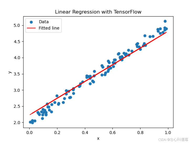
练习2：线性拟合(不需要自己写前向和反向传播计算)

import numpy as np
import tensorflow as tf
from tensorflow.keras.models import Sequential
from tensorflow.keras.layers import Dense
import matplotlib.pyplot as plt
from tensorflow.keras.optimizers import Adam



'''
hh1.py相比hh.py，抽象程度更高
'''


def main():
    # 生成一些带有噪声的一次函数数据
    np.random.seed(42)
    X = np.linspace(-1, 1, 100)[:, np.newaxis]  # 生成100个等间距的x值
    noise = np.random.normal(0, 0.1, X.shape)  # 添加一些高斯噪声
    y = 2 * X + 1 + noise  # 生成y值，假设真实关系是 y=2x+1

    # 创建一个简单的线性回归模型（1层）
    model = Sequential([
        Dense(1, input_shape=(1,), activation='linear')
    ])




    # ----------------------------------------------------------
    # 编译模型，使用均方误差作为损失函数
    model.compile(optimizer=Adam(learning_rate=0.01), loss='mse')

    # 训练模型
    history = model.fit(X, y, epochs=500, verbose=0)

    # 使用训练好的模型进行预测
    y_pred = model.predict(X)
    # ----------------------------------------------------------




    # 绘制结果
    plt.figure(figsize=(8, 6))
    plt.scatter(X, y, color='blue', label='Data')  # 原始数据点
    plt.plot(X, y_pred, color='red', label='Fitted line')  # 拟合的直线
    plt.title('Linear Regression with TensorFlow/Keras')
    plt.xlabel('X')
    plt.ylabel('y')
    plt.legend()
    plt.show()

    # 打印最终的权重和偏置
    weights, bias = model.get_weights()
    print(f'Weight: {weights[0][0]}, Bias: {bias[0]}')

if __name__ == '__main__':
    main()

         \;\\\;\\\;

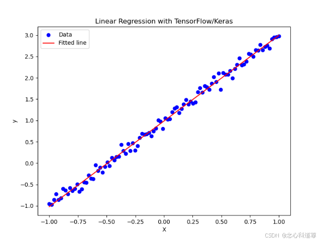
练习3：二次曲线拟合

import numpy as np
import tensorflow as tf
from tensorflow.keras.models import Sequential
from tensorflow.keras.layers import Dense
import matplotlib.pyplot as plt



'''
预测二次函数，使用三层MLP模型
'''


def main():
    # 生成带有噪声的二次函数数据
    np.random.seed(42)
    X = np.linspace(-2, 2, 100)[:, np.newaxis]  # 生成100个等间距的x值
    noise = np.random.normal(0, 0.5, X.shape)   # 添加一些高斯噪声

    y = 1 * X**2 + 2 * X + 3 + noise            # 生成y值，假设真实关系是 y=x^2 + 2x + 3

    # 创建一个MLP模型（3层）
    model = Sequential([
        Dense(16, input_shape=(1,), activation='relu'),  # 隐藏层，使用ReLU激活函数
        Dense(8, activation='relu'),                     # 隐藏层
        Dense(1, activation='linear')                    # 输出层，使用线性激活函数
    ])



    #----------------------------------------------------------
    # 编译模型，使用均方误差作为损失函数
    model.compile(optimizer=tf.keras.optimizers.Adam(learning_rate=0.01), loss='mse')

    # 训练模型
    history = model.fit(X, y, epochs=1000, verbose=0)

    # 使用训练好的模型进行预测
    y_pred = model.predict(X)
    # ----------------------------------------------------------



    # 绘制结果
    plt.figure(figsize=(8, 6))
    plt.scatter(X, y, color='blue', label='Data')  # 原始数据点
    plt.plot(X, y_pred, color='red', label='Fitted curve')  # 拟合的曲线
    plt.title('Quadratic Function Fitting with MLP (TensorFlow/Keras)')
    plt.xlabel('X')
    plt.ylabel('y')
    plt.legend()
    plt.show()

if __name__ == '__main__':
    main()

         \;\\\;\\\;

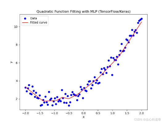
练习4：RNN预测拟合

# -*- coding:utf-8 -*-
# 2024/12/28 hh3.py Yishijun

'''
时间序列预测：RNN、LSTM、GRU
'''

import numpy as np
import pandas as pd
import matplotlib.pyplot as plt
from sklearn.preprocessing import MinMaxScaler
from tensorflow.keras.models import Sequential
from tensorflow.keras.layers import SimpleRNN, Dense
from tensorflow.keras.optimizers import Adam


def generate_sine_wave(num_samples=1000):
    # 生成带有噪声的正弦波数据作为时间序列
    time = np.linspace(0, 10, num_samples)  # 创建等间距的时间点
    data = np.sin(time) + np.random.normal(0.1, 0.2, num_samples)  # 正弦波加上随机噪声
    return data


def create_dataset(data, time_steps=10):
    # 创建滑动窗口形式的数据集，每个输入序列包含过去time_steps个时间点的数据
    X, y = [], []
    for i in range(len(data) - time_steps):
        X.append(data[i:i + time_steps])  # 输入序列
        y.append(data[i + time_steps])  # 对应的目标值（下一个时间点的值）
    return np.array(X), np.array(y)


def Main():
    # 生成数据
    data = generate_sine_wave()

    # 数据标准化
    scaler = MinMaxScaler(feature_range=(0, 1))  # 定义归一化范围为[0, 1]
    scaled_data = scaler.fit_transform(data.reshape(-1, 1))  # 将数据转换成二维数组并进行归一化

    # 创建输入-输出对
    time_steps = 10  # 使用过去10个时间步长来预测下一个值
    X, y = create_dataset(scaled_data, time_steps)

    # 将数据分为训练集50%和测试集50%
    split = int(0.5 * len(X))
    X_train, X_test = X[:split], X[split:]
    y_train, y_test = y[:split], y[split:]

    # 调整输入形状以适应RNN
    X_train = X_train.reshape((X_train.shape[0], X_train.shape[1], 1))  # [样本数, 时间步, 特征数]
    X_test = X_test.reshape((X_test.shape[0], X_test.shape[1], 1))

    # 构建RNN模型
    model = Sequential([
        SimpleRNN(50, activation='relu', input_shape=(time_steps, 1)),  # RNN层，50个单元
        Dense(1)  # 输出层，单个神经元用于回归问题
    ])

    # ----------------------------------------------------------
    # 编译模型
    model.compile(optimizer=Adam(learning_rate=0.01), loss='mean_squared_error')  # 使用均方误差作为损失函数

    # 打印模型摘要
    model.summary()  # 显示模型结构和参数量

    # 训练模型
    history = model.fit(X_train, y_train, epochs=20, batch_size=32, validation_data=(X_test, y_test))  # 训练20个周期

    # 进行预测
    y_pred = model.predict(X_test)  # 使用测试集数据进行预测

    # 反向标准化预测结果
    y_pred = scaler.inverse_transform(y_pred)  # 将预测结果从归一化的值转换回原始值
    y_test = scaler.inverse_transform(y_test.reshape(-1, 1))  # 同样将y_test反向标准化

    # 反向标准化训练集和测试集的实际值
    y_train_inv = scaler.inverse_transform(y_train.reshape(-1, 1))  # 训练集目标值反向标准化
    y_test_inv = scaler.inverse_transform(y_test.reshape(-1, 1))  # 测试集目标值反向标准化
    # ----------------------------------------------------------

    # 绘制预测结果
    plt.figure(figsize=(10, 6))

    # 绘制完整的时间序列（包括训练集和测试集）
    plt.plot(np.arange(len(data)), data, color='gray', alpha=0.5, label='Original Data')  # 原始数据用灰色表示

    # 绘制训练集部分（蓝色）
    train_start = time_steps  # 训练集从第time_steps个时间点开始
    train_end = train_start + len(y_train)
    plt.plot(np.arange(train_start, train_end), y_train_inv, color='blue', label='Training Set')  # 训练集真实值

    # # 绘制测试集部分（绿色）
    test_start = train_end
    test_end = test_start + len(y_test)
    # plt.plot(np.arange(test_start, test_end), y_test_inv, color='green', label='Test Set (True)')  # 注释掉了绘制测试集真实值的代码，因为y_test不是原本值了

    # 绘制预测结果（红色虚线）
    plt.plot(np.arange(test_start, test_end), y_pred, color='red', linestyle='--', label='Predicted')  # 预测值

    # 添加标题和标签
    plt.title('RNN Prediction vs Actual')
    plt.xlabel('Time Step')
    plt.ylabel('Value')

    # 显示图例
    plt.legend()

    # 显示图表
    plt.show()

    # 调试输出，用于检查时间轴和数据的一致性
    print("Train Start Index:", train_start)
    print("Train End Index:", train_end)
    print("Test Start Index:", test_start)
    print("Test End Index:", test_end)
    print("Shape of y_test_inv:", y_test_inv.shape)
    print("First few values of original data in test set:")
    print(data[test_start:test_start+5])
    print("First few values of y_test_inv:")
    print(y_test_inv[:5])

if __name__ == '__main__':
    Main()

         \;\\\;\\\;

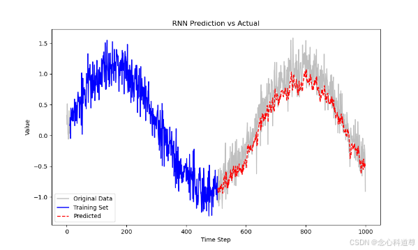
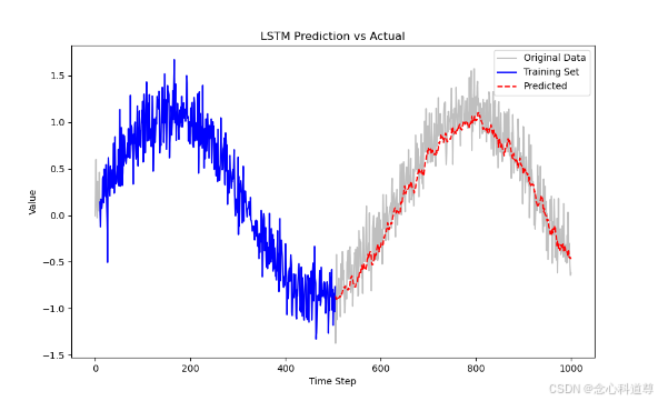
练习5：LSTM预测拟合

# -*- coding:utf-8 -*-
# 2024/12/28 hh3.py Yishijun

'''
时间序列预测：LSTM
'''

import numpy as np
import pandas as pd
import matplotlib.pyplot as plt
from sklearn.preprocessing import MinMaxScaler
from tensorflow.keras.models import Sequential
from tensorflow.keras.layers import LSTM, Dense
from tensorflow.keras.optimizers import Adam


def generate_sine_wave(num_samples=1000):
    # 生成带有噪声的正弦波数据作为时间序列
    time = np.linspace(0, 10, num_samples)  # 创建等间距的时间点
    data = np.sin(time) + np.random.normal(0.1, 0.2, num_samples)  # 正弦波加上随机噪声
    return data


def create_dataset(data, time_steps=10):
    # 创建滑动窗口形式的数据集，每个输入序列包含过去time_steps个时间点的数据
    X, y = [], []
    for i in range(len(data) - time_steps):
        X.append(data[i:i + time_steps])  # 输入序列
        y.append(data[i + time_steps])  # 对应的目标值（下一个时间点的值）
    return np.array(X), np.array(y)


def Main():
    # 生成数据
    data = generate_sine_wave()

    # 数据标准化
    scaler = MinMaxScaler(feature_range=(0, 1))  # 定义归一化范围为[0, 1]
    scaled_data = scaler.fit_transform(data.reshape(-1, 1))  # 将数据转换成二维数组并进行归一化

    # 创建输入-输出对
    time_steps = 10  # 使用过去10个时间步长来预测下一个值
    X, y = create_dataset(scaled_data, time_steps)

    # 将数据分为训练集50%和测试集50%
    split = int(0.5 * len(X))
    X_train, X_test = X[:split], X[split:]
    y_train, y_test = y[:split], y[split:]

    # 调整输入形状以适应LSTM
    X_train = X_train.reshape((X_train.shape[0], X_train.shape[1], 1))  # [样本数, 时间步, 特征数]
    X_test = X_test.reshape((X_test.shape[0], X_test.shape[1], 1))

    # 构建LSTM模型
    model = Sequential([
        LSTM(50, activation='relu', input_shape=(time_steps, 1)),  # LSTM层，50个单元
        Dense(1)  # 输出层，单个神经元用于回归问题
    ])

    # 编译模型
    model.compile(optimizer=Adam(learning_rate=0.01), loss='mean_squared_error')  # 使用均方误差作为损失函数

    # 打印模型摘要
    model.summary()  # 显示模型结构和参数量

    # 训练模型
    history = model.fit(X_train, y_train, epochs=20, batch_size=32, validation_data=(X_test, y_test))  # 训练20个周期

    # 进行预测
    y_pred = model.predict(X_test)  # 使用测试集数据进行预测

    # 反向标准化预测结果
    y_pred = scaler.inverse_transform(y_pred)  # 将预测结果从归一化的值转换回原始值
    y_test = scaler.inverse_transform(y_test.reshape(-1, 1))  # 同样将y_test反向标准化

    # 反向标准化训练集和测试集的实际值
    y_train_inv = scaler.inverse_transform(y_train.reshape(-1, 1))  # 训练集目标值反向标准化
    y_test_inv = scaler.inverse_transform(y_test.reshape(-1, 1))  # 测试集目标值反向标准化

    # 绘制预测结果
    plt.figure(figsize=(10, 6))

    # 绘制完整的时间序列（包括训练集和测试集）
    plt.plot(np.arange(len(data)), data, color='gray', alpha=0.5, label='Original Data')  # 原始数据用灰色表示

    # 绘制训练集部分（蓝色）
    train_start = time_steps  # 训练集从第time_steps个时间点开始
    train_end = train_start + len(y_train)
    plt.plot(np.arange(train_start, train_end), y_train_inv, color='blue', label='Training Set')  # 训练集真实值

    # 绘制测试集部分（绿色）
    test_start = train_end
    test_end = test_start + len(y_test)
    #plt.plot(np.arange(test_start, test_end), y_test_inv, color='green', label='Test Set (True)')  # 测试集真实值

    # 绘制预测结果（红色虚线）
    plt.plot(np.arange(test_start, test_end), y_pred, color='red', linestyle='--', label='Predicted')  # 预测值

    # 添加标题和标签
    plt.title('LSTM Prediction vs Actual')
    plt.xlabel('Time Step')
    plt.ylabel('Value')

    # 显示图例
    plt.legend()

    # 显示图表
    plt.show()

    # 调试输出，用于检查时间轴和数据的一致性
    print("Train Start Index:", train_start)
    print("Train End Index:", train_end)
    print("Test Start Index:", test_start)
    print("Test End Index:", test_end)
    print("Shape of y_test_inv:", y_test_inv.shape)
    print("First few values of original data in test set:")
    print(data[test_start:test_start+5])
    print("First few values of y_test_inv:")
    print(y_test_inv[:5])

if __name__ == '__main__':
    Main()

         \;\\\;\\\;

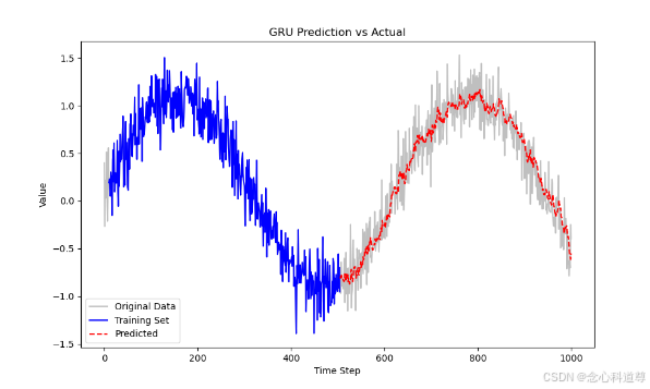
练习6：GRU预测拟合

# -*- coding:utf-8 -*-
# 2024/12/28 hh3.py Yishijun

'''
时间序列预测：GRU
'''

import numpy as np
import pandas as pd
import matplotlib.pyplot as plt
from sklearn.preprocessing import MinMaxScaler
from tensorflow.keras.models import Sequential
from tensorflow.keras.layers import GRU, Dense
from tensorflow.keras.optimizers import Adam


def generate_sine_wave(num_samples=1000):
    # 生成带有噪声的正弦波数据作为时间序列
    time = np.linspace(0, 10, num_samples)  # 创建等间距的时间点
    data = np.sin(time) + np.random.normal(0.1, 0.2, num_samples)  # 正弦波加上随机噪声
    return data


def create_dataset(data, time_steps=10):
    # 创建滑动窗口形式的数据集，每个输入序列包含过去time_steps个时间点的数据
    X, y = [], []
    for i in range(len(data) - time_steps):
        X.append(data[i:i + time_steps])  # 输入序列
        y.append(data[i + time_steps])  # 对应的目标值（下一个时间点的值）
    return np.array(X), np.array(y)


def Main():
    # 生成数据
    data = generate_sine_wave()

    # 数据标准化
    scaler = MinMaxScaler(feature_range=(0, 1))  # 定义归一化范围为[0, 1]
    scaled_data = scaler.fit_transform(data.reshape(-1, 1))  # 将数据转换成二维数组并进行归一化

    # 创建输入-输出对
    time_steps = 10  # 使用过去10个时间步长来预测下一个值
    X, y = create_dataset(scaled_data, time_steps)

    # 将数据分为训练集50%和测试集50%
    split = int(0.5 * len(X))
    X_train, X_test = X[:split], X[split:]
    y_train, y_test = y[:split], y[split:]

    # 调整输入形状以适应GRU
    X_train = X_train.reshape((X_train.shape[0], X_train.shape[1], 1))  # [样本数, 时间步, 特征数]
    X_test = X_test.reshape((X_test.shape[0], X_test.shape[1], 1))

    # 构建GRU模型
    model = Sequential([
        GRU(50, activation='relu', input_shape=(time_steps, 1)),  # GRU层，50个单元
        Dense(1)  # 输出层，单个神经元用于回归问题
    ])

    # 编译模型
    model.compile(optimizer=Adam(learning_rate=0.01), loss='mean_squared_error')  # 使用均方误差作为损失函数

    # 打印模型摘要
    model.summary()  # 显示模型结构和参数量

    # 训练模型
    history = model.fit(X_train, y_train, epochs=20, batch_size=32, validation_data=(X_test, y_test))  # 训练20个周期

    # 进行预测
    y_pred = model.predict(X_test)  # 使用测试集数据进行预测

    # 反向标准化预测结果
    y_pred = scaler.inverse_transform(y_pred)  # 将预测结果从归一化的值转换回原始值
    y_test = scaler.inverse_transform(y_test.reshape(-1, 1))  # 同样将y_test反向标准化

    # 反向标准化训练集和测试集的实际值
    y_train_inv = scaler.inverse_transform(y_train.reshape(-1, 1))  # 训练集目标值反向标准化
    y_test_inv = scaler.inverse_transform(y_test.reshape(-1, 1))  # 测试集目标值反向标准化

    # 绘制预测结果
    plt.figure(figsize=(10, 6))

    # 绘制完整的时间序列（包括训练集和测试集）
    plt.plot(np.arange(len(data)), data, color='gray', alpha=0.5, label='Original Data')  # 原始数据用灰色表示

    # 绘制训练集部分（蓝色）
    train_start = time_steps  # 训练集从第time_steps个时间点开始
    train_end = train_start + len(y_train)
    plt.plot(np.arange(train_start, train_end), y_train_inv, color='blue', label='Training Set')  # 训练集真实值

    # 绘制测试集部分（绿色）
    test_start = train_end
    test_end = test_start + len(y_test)
    #plt.plot(np.arange(test_start, test_end), y_test_inv, color='green', label='Test Set (True)')  # 测试集真实值

    # 绘制预测结果（红色虚线）
    plt.plot(np.arange(test_start, test_end), y_pred, color='red', linestyle='--', label='Predicted')  # 预测值

    # 添加标题和标签
    plt.title('GRU Prediction vs Actual')
    plt.xlabel('Time Step')
    plt.ylabel('Value')

    # 显示图例
    plt.legend()

    # 显示图表
    plt.show()

    # 调试输出，用于检查时间轴和数据的一致性
    print("Train Start Index:", train_start)
    print("Train End Index:", train_end)
    print("Test Start Index:", test_start)
    print("Test End Index:", test_end)
    print("Shape of y_test_inv:", y_test_inv.shape)
    print("First few values of original data in test set:")
    print(data[test_start:test_start+5])
    print("First few values of y_test_inv:")
    print(y_test_inv[:5])

if __name__ == '__main__':
    Main()

         \;\\\;\\\;

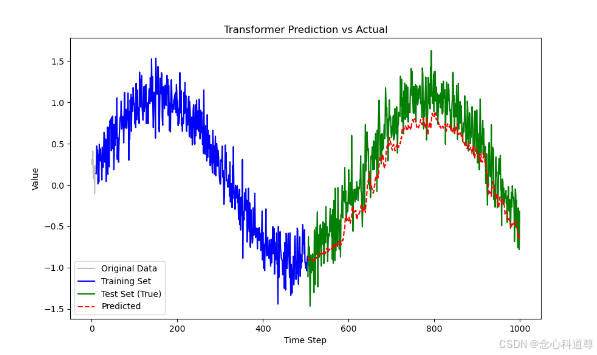
练习7：Transformer预测拟合

import numpy as np
import pandas as pd
import matplotlib.pyplot as plt
from sklearn.preprocessing import MinMaxScaler
import tensorflow as tf
from tensorflow.keras.models import Model
from tensorflow.keras.layers import Input, Dense, LayerNormalization, Dropout, MultiHeadAttention, \
    GlobalAveragePooling1D
from tensorflow.keras.optimizers import Adam


# 1. 生成带有噪声的正弦波数据
def generate_sine_wave(num_samples=1000):
    time = np.linspace(0, 10, num_samples)  # 创建等间距的时间点
    data = np.sin(time) + np.random.normal(0.1, 0.2, num_samples)  # 正弦波加上随机噪声
    return data


# 2. 创建滑动窗口数据集
def create_dataset(data, time_steps=10):
    X, y = [], []
    for i in range(len(data) - time_steps):
        X.append(data[i:i + time_steps])  # 输入序列
        y.append(data[i + time_steps])  # 对应的目标值（下一个时间点的值）
    return np.array(X), np.array(y)


# 3. 定义位置编码层
class PositionalEncoding(tf.keras.layers.Layer):
    def __init__(self, position, d_model):
        super(PositionalEncoding, self).__init__()
        self.pos_encoding = self.positional_encoding(position, d_model)

    def get_angles(self, position, i, d_model):
        angles = 1 / np.power(10000, (2 * (i // 2)) / np.float32(d_model))
        return position * angles

    def positional_encoding(self, position, d_model):
        angle_rads = self.get_angles(
            np.arange(position)[:, np.newaxis],
            np.arange(d_model)[np.newaxis, :],
            d_model
        )
        # apply sin to even indices in the array; 2i
        angle_rads[:, 0::2] = np.sin(angle_rads[:, 0::2])
        # apply cos to odd indices in the array; 2i+1
        angle_rads[:, 1::2] = np.cos(angle_rads[:, 1::2])
        pos_encoding = angle_rads[np.newaxis, ...]
        return tf.cast(pos_encoding, dtype=tf.float32)

    def call(self, inputs):
        return inputs + self.pos_encoding[:, :tf.shape(inputs)[1], :]


# 4. 定义Transformer块
class TransformerBlock(tf.keras.layers.Layer):
    def __init__(self, embed_dim, num_heads, ff_dim, rate=0.1):
        super(TransformerBlock, self).__init__()
        self.att = MultiHeadAttention(num_heads=num_heads, key_dim=embed_dim)
        self.ffn = tf.keras.Sequential([
            Dense(ff_dim, activation="relu"),  # 前馈神经网络的第一层
            Dense(embed_dim)  # 前馈神经网络的第二层
        ])
        self.layernorm1 = LayerNormalization(epsilon=1e-6)
        self.layernorm2 = LayerNormalization(epsilon=1e-6)
        self.dropout1 = Dropout(rate)
        self.dropout2 = Dropout(rate)

    def call(self, inputs, training):
        attn_output = self.att(inputs, inputs)
        attn_output = self.dropout1(attn_output, training=training)
        out1 = self.layernorm1(inputs + attn_output)
        ffn_output = self.ffn(out1)
        ffn_output = self.dropout2(ffn_output, training=training)
        return self.layernorm2(out1 + ffn_output)


# 5. 构建Transformer模型
def build_transformer_model(input_shape, embed_dim, num_heads, ff_dim, num_layers):
    inputs = Input(shape=input_shape)

    # 添加位置编码
    x = PositionalEncoding(input_shape[0], embed_dim)(inputs)

    # 添加多个Transformer块
    for _ in range(num_layers):
        x = TransformerBlock(embed_dim, num_heads, ff_dim)(x)

    # 全局平均池化
    x = GlobalAveragePooling1D()(x)

    # 全连接层
    x = Dense(20, activation="relu")(x)
    x = Dropout(0.1)(x)

    # 输出层
    outputs = Dense(1)(x)

    model = Model(inputs=inputs, outputs=outputs)
    return model







# 6. 主函数
def main():
    # 生成数据
    data = generate_sine_wave()

    # 数据标准化
    scaler = MinMaxScaler(feature_range=(0, 1))
    scaled_data = scaler.fit_transform(data.reshape(-1, 1))

    # 定义时间步长
    time_steps = 10  # 使用过去10个时间步长来预测下一个值

    # 创建输入-输出对
    X, y = create_dataset(scaled_data, time_steps)

    # 将数据分为训练集50%和测试集50%
    split = int(0.5 * len(X))
    X_train, X_test = X[:split], X[split:]
    y_train, y_test = y[:split], y[split:]

    # 调整输入形状以适应Transformer
    X_train = X_train.reshape((X_train.shape[0], X_train.shape[1], 1))  # [样本数, 时间步, 特征数]
    X_test = X_test.reshape((X_test.shape[0], X_test.shape[1], 1))

    # 构建Transformer模型
    input_shape = (time_steps, 1)  # 输入形状为 [时间步, 特征数]
    embed_dim = 32  # 嵌入维度
    num_heads = 4  # 多头注意力机制的头数
    ff_dim = 32  # 前馈神经网络的隐藏层维度
    num_layers = 2  # Transformer块的数量

    model = build_transformer_model(input_shape, embed_dim, num_heads, ff_dim, num_layers)

    # 编译模型
    model.compile(optimizer=Adam(learning_rate=0.001), loss='mean_squared_error')

    # 打印模型摘要
    model.summary()

    # 训练模型
    history = model.fit(
        X_train, y_train,
        epochs=20,
        batch_size=32,
        validation_data=(X_test, y_test),
        verbose=1
    )

    # 进行预测
    y_pred = model.predict(X_test)

    # 反向标准化预测结果
    y_pred = scaler.inverse_transform(y_pred)
    y_test = scaler.inverse_transform(y_test.reshape(-1, 1))

    # 绘制预测结果
    plt.figure(figsize=(10, 6))

    # 绘制完整的时间序列（包括训练集和测试集）
    plt.plot(np.arange(len(data)), data, color='gray', alpha=0.5, label='Original Data')  # 原始数据用灰色表示

    # 绘制训练集部分（蓝色）
    train_start = time_steps  # 训练集从第time_steps个时间点开始
    train_end = train_start + len(y_train)
    plt.plot(np.arange(train_start, train_end), scaler.inverse_transform(y_train.reshape(-1, 1)), color='blue',
             label='Training Set')  # 训练集真实值

    # 绘制测试集部分（绿色）
    test_start = train_end
    test_end = test_start + len(y_test)
    plt.plot(np.arange(test_start, test_end), y_test, color='green', label='Test Set (True)')  # 测试集真实值

    # 绘制预测结果（红色虚线）
    plt.plot(np.arange(test_start, test_end), y_pred, color='red', linestyle='--', label='Predicted')  # 预测值

    # 添加标题和标签
    plt.title('Transformer Prediction vs Actual')
    plt.xlabel('Time Step')
    plt.ylabel('Value')

    # 显示图例
    plt.legend()

    # 显示图表
    plt.show()


if __name__ == '__main__':
    main()

         \;\\\;\\\;

练习8：MLP+RNN预测拟合

import numpy as np
import pandas as pd
import tensorflow as tf
from tensorflow.keras.models import Model
from tensorflow.keras.layers import Input, Dense, LSTM, concatenate
from sklearn.model_selection import train_test_split
from sklearn.preprocessing import StandardScaler
import matplotlib.pyplot as plt
from statsmodels.tsa.seasonal import seasonal_decompose
from scipy.signal import sawtooth  # 用于生成锯齿波（模拟季节性）

# 2. 生成时间序列数据
def generate_time_series_data(num_samples, time_steps, num_features):
    """
    生成包含长期大趋势、短期小趋势、自回归项和随机游走的时间序列数据。

    参数:
    - num_samples: 样本数量
    - time_steps: 每个样本的时间步长
    - num_features: 每个时间步的特征数

    返回:
    - X_time: 生成的时间序列数据，形状为 (num_samples, time_steps, num_features)
    """
    # 生成长期大趋势（指数增长或衰减）
    trend = np.exp(np.linspace(0, 2, time_steps)) * 5  # 指数增长趋势

    # 生成短期小趋势（使用正弦波模拟）
    short_trend = np.sin(2 * np.pi * 0.05 * np.arange(time_steps))  # 短期周期性波动

    # 生成自回归项（当前值依赖于前一个值）
    ar_term = np.zeros(time_steps)
    for t in range(1, time_steps):
        ar_term[t] = 0.8 * ar_term[t-1] + np.random.normal(0, 0.1)

    # 生成随机游走项
    random_walk = np.cumsum(np.random.normal(0, 0.1, size=time_steps))

    # 生成噪声（随机扰动）
    noise = np.random.normal(0, 0.1, size=(num_samples, time_steps, num_features))

    # 生成时间序列数据
    X_time = np.zeros((num_samples, time_steps, num_features))
    for i in range(num_samples):
        for j in range(num_features):
            X_time[i, :, j] = trend + short_trend + ar_term + random_walk + noise[i, :, j]

    return X_time


# 生成静态特征
def generate_static_features(num_samples, num_static_features):
    """
    生成包含相关性的静态特征数据。

    参数:
    - num_samples: 样本数量
    - num_static_features: 静态特征的数量

    返回:
    - X_static: 生成的静态特征数据，形状为 (num_samples, num_static_features)
    """
    # 生成随机静态特征
    X_static = np.random.randn(num_samples, num_static_features)

    # 添加一些相关性（例如，市值与市盈率之间的正相关）
    X_static[:, 0] = np.abs(X_static[:, 0])  # 市值为正值
    X_static[:, 1] = X_static[:, 0] * (1 + np.random.normal(0, 0.2, size=num_samples))  # 市盈率与市值相关

    return X_static


# 生成目标值（未来股票价格）
def generate_target_values(X_time, X_static, num_samples):
    """
    生成基于时间序列数据和静态特征的目标值（未来股票价格）。

    参数:
    - X_time: 时间序列数据，形状为 (num_samples, time_steps, num_features)
    - X_static: 静态特征数据，形状为 (num_samples, num_static_features)
    - num_samples: 样本数量

    返回:
    - y: 生成的目标值，形状为 (num_samples, 1)
    """
    # 目标值基于时间序列数据的最后一个时间步的价格，并结合静态特征的影响
    # 还考虑了过去几个时间步的价格变化率和波动率
    last_price = X_time[:, -1, 0]
    price_change_rate = (X_time[:, -1, 0] - X_time[:, -2, 0]) / X_time[:, -2, 0]
    volatility = np.std(X_time[:, -5:, 0], axis=1)  # 最近5个时间步的波动率

    y = last_price + 0.5 * price_change_rate + 0.1 * volatility + np.sum(X_static, axis=1) * 0.01 + np.random.normal(0, 0.1, size=num_samples)
    return y.reshape(-1, 1)


# 4. 定义RNN模块
def build_rnn_module(input_shape):
    """
    构建RNN模块，用于处理时间序列数据。

    参数:
    - input_shape: 输入数据的形状 (time_steps, num_features)

    返回:
    - input_time: RNN模块的输入层
    - rnn_output: RNN模块的输出层
    """
    input_time = Input(shape=input_shape, name='input_time')
    lstm_output = LSTM(64, return_sequences=False)(input_time)  # 返回最后一个时间步的输出
    rnn_output = Dense(32, activation='relu')(lstm_output)
    return input_time, rnn_output


# 5. 定义MLP模块
def build_mlp_module(input_shape):
    """
    构建MLP模块，用于处理静态特征。

    参数:
    - input_shape: 输入数据的形状 (num_static_features,)

    返回:
    - input_static: MLP模块的输入层
    - mlp_output: MLP模块的输出层
    """
    input_static = Input(shape=input_shape, name='input_static')
    dense1 = Dense(64, activation='relu')(input_static)
    dense2 = Dense(32, activation='relu')(dense1)
    return input_static, dense2


# 6. 定义融合模块
def build_fusion_module(rnn_output, mlp_output):
    """
    构建融合模块，将RNN模块和MLP模块的输出拼接在一起，并进行最终的回归预测。

    参数:
    - rnn_output: RNN模块的输出层
    - mlp_output: MLP模块的输出层

    返回:
    - output: 融合模块的输出层
    """
    concatenated = concatenate([rnn_output, mlp_output])
    fusion_output = Dense(32, activation='relu')(concatenated)
    output = Dense(1, activation='linear')(fusion_output)  # 回归任务，使用线性激活函数
    return output


# 7. 构建完整模型
def build_hybrid_model(time_input_shape, static_input_shape):
    """
    构建完整的混合模型，包含RNN模块、MLP模块和融合模块。

    参数:
    - time_input_shape: 时间序列数据的输入形状 (time_steps, num_features)
    - static_input_shape: 静态特征的输入形状 (num_static_features,)

    返回:
    - model: 构建好的混合模型
    """
    input_time, rnn_output = build_rnn_module(time_input_shape)
    input_static, mlp_output = build_mlp_module(static_input_shape)
    output = build_fusion_module(rnn_output, mlp_output)
    model = Model(inputs=[input_time, input_static], outputs=output)
    return model


def main():
    # 1. 数据准备

    # 设置随机种子以确保结果可复现
    np.random.seed(42)

    # 定义数据参数
    time_steps = 60  # 每个样本的时间步长
    num_features = 5  # 每个时间步的特征数（如价格、成交量等）
    num_static_features = 8  # 静态特征的数量（如公司市值、市盈率等）
    num_samples = 50000  # 增加样本数量

    # 生成数据
    X_time = generate_time_series_data(num_samples, time_steps, num_features)
    X_static = generate_static_features(num_samples, num_static_features)
    y = generate_target_values(X_time, X_static, num_samples)

    # 3. 数据预处理
    # 将数据分为训练集和测试集
    X_train_time, X_test_time, X_train_static, X_test_static, y_train, y_test = train_test_split(
        X_time, X_static, y, test_size=0.2, random_state=42
    )

    # 对静态特征进行标准化
    scaler = StandardScaler()
    X_train_static = scaler.fit_transform(X_train_static)
    X_test_static = scaler.transform(X_test_static)

    # 8. 编译和训练模型
    time_input_shape = (time_steps, num_features)
    static_input_shape = (num_static_features,)

    model = build_hybrid_model(time_input_shape, static_input_shape)

    # 编译模型
    model.compile(optimizer='adam', loss='mean_squared_error', metrics=['mae'])

    # 打印模型摘要
    model.summary()

    # 训练模型
    history = model.fit(
        [X_train_time, X_train_static], y_train,
        epochs=50,
        batch_size=32,
        validation_data=([X_test_time, X_test_static], y_test),
        verbose=1
    )

    # 9. 评估模型
    test_loss, test_mae = model.evaluate([X_test_time, X_test_static], y_test)
    print(f"Test Loss: {test_loss:.4f}")
    print(f"Test MAE: {test_mae:.4f}")

    # 10. 绘制训练和验证的损失曲线
    plt.plot(history.history['loss'], label='Train Loss')
    plt.plot(history.history['val_loss'], label='Validation Loss')
    plt.title('Model Loss')
    plt.xlabel('Epochs')
    plt.ylabel('Loss')
    plt.legend()
    plt.show()

    # 11. 预测并可视化结果
    predictions = model.predict([X_test_time, X_test_static])

    # 可视化前100个样本的真实值与预测值
    plt.figure(figsize=(10, 6))
    plt.plot(y_test[:100], label='True Values', marker='o')
    plt.plot(predictions[:100], label='Predicted Values', marker='x')
    plt.title('True vs Predicted Stock Prices')
    plt.xlabel('Sample Index')
    plt.ylabel('Stock Price')
    plt.legend()
    plt.show()

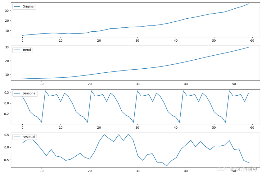
    # 12. 可视化时间序列数据的趋势和季节性
    sample_index = 0  # 选择一个样本进行可视化
    sample_data = X_time[sample_index, :, 0]

    # 使用statsmodels分解时间序列
    result = seasonal_decompose(sample_data, period=12, model='additive')

    # 绘制分解结果
    plt.figure(figsize=(12, 8))
    plt.subplot(411)
    plt.plot(sample_data, label='Original')
    plt.legend(loc='upper left')
    plt.subplot(412)
    plt.plot(result.trend, label='Trend')
    plt.legend(loc='upper left')
    plt.subplot(413)
    plt.plot(result.seasonal, label='Seasonal')
    plt.legend(loc='upper left')
    plt.subplot(414)
    plt.plot(result.resid, label='Residual')
    plt.legend(loc='upper left')
    plt.tight_layout()
    plt.show()


if __name__ == '__main__':
    main()

         \;\\\;\\\;