文章源代码https://github.com/tilmto/autoai2c

原论文：Yongan Zhang, Xiaofan Zhang et al. AutoAI2C: An Automated Hardware Generator for DNN Acceleration on Both FPGA and ASIC. IEEE Transactions on Computer-aided Design of Integrated Circuits and Systems, vol. 43, no. 10, October 2024.

1 引言

        随着数据需求的增长以及硬件算力性能的提升,人工智能得到越来越广泛的应用。其中, 神经网络算法已经被成功地用于解决一些实际问题。尽管这些算法有着卓越的表现, 但其在传统硬件平台上的计算性能仍然不够高效。因此，DNN加速器可以根据不同的神经网络架构定制化地设计加速器，从而加速运算和处理地速度。

        通常来看，DNN加速器的实现主要有以下几种：依赖于一组预先选择的数据维度来利用处理元件（PE）阵列上的高并行性以实现高性能和数据重用以实现高能效；通过空间架构（如脉动阵列）或分布式计算提升吞吐量；使用片上网络（NoC）或灵活的数据通路，根据计算需求动态调度数据，避免拥塞。

关于DNN加速器设计方法的研究已经取得了显著进展。有学者已经提出一种自动设计DNN加速器的方法：AutoAI2C[1]。探索设计空间时，通过一种面向对象的基于图形的表示，它统一了三个抽象层次的设计因素 ：IP、架构和硬件映射。首先使用PE阵列架构、内存架构和映射/数据流的设计因素构建一个基本的有向图，并给出了有向图中能量，延迟，内存容量的计算方式。根据操作依赖性和算法映射，ip在图上的邻居IP分别被指定为ip.prev和ip.next，根据预先定义的StM属性，为每个实例化的IP建立StM，以存储整个执行过程中的不同状态。此外，借助遗传算法（EA），从初始的硬件配置种群开始，每一代通过选择、交叉、变异等方式产生新的硬件配置。

        此外，有学者提出了Eyeriss v2 [2] DNN加速器架构。针对片上网络中数据层的形状和大小变化较大的问题，提出了一种高度灵活的片上网络——分层网格，能够适应不同数据类型的数据复用量和带宽需求，提高了计算资源的利用率。

本文对遗传算法和设计空间探索的过程进行验证，模拟执行的过程。对DNN加速器的HLS C代码进行了综合和FPGA上版以验证其有效性，评估是否可以对神经网络进行加速及其加速效果，以便对其性能做出进一步的优化。

2 实验内容

        AutoAI2C的代码[3]被用来模拟整个遗传算法，从硬件IP池中生成常用和适用于AlexNet的硬件架构模板和硬件IP模板，进行硬件配置的快速探索，由于本地的运算能力有限，最大种群数设为10。在第一阶段的DSE中，得到40个硬件的评分如图1所示。

其中，最优得分为-69.52795318613326，对应四个硬件参数：gb_vol: 786432, rf_vol: 3072, num_pe: 256, num_rf: 256，和作者得到的一致。将这个配置参数送入第二阶段的DSE，进行IP优化，得到每一层的片上互连模板，寻找循环顺序和分块因素。

按照传统的FPGA工程链路，对作者给出的单通道卷积HLS代码进行了测试。使用Vitis 2024.2进行了综合，生成IP核。使用的资源如表1所示，延时为3.67s。使用Vivado 2024.2 对IP核电路连接进行构建，生成位流文件。

	Syn	PnR
LUT	5719	5325
FF	6306	9566
DSP	29	29
SRL	429	247
BRAM	36	36
SLICE	0	3772

表1.单通道 HLS综合时的资源使用情况

    在PYNQ平台实现加速模型时，两种IP核和PS的连接方式经过了实验。第一种结构是通过DMA进行传输，第二种结构是直接通过m_axi进行读写，存储在片外储存器（DDR3），如图2所示。第一种设计并未成功。在实验中完成传输后读出的值全部为0。利用vivado的ILA抓取信号发现tvaild没有置1，原因是源代码没有采用stream方式读取数据，所以传输失败。第二种结构完成了数据的读取和卷积的计算，计算时间为17.85s，单张图片的FPS为0.06。

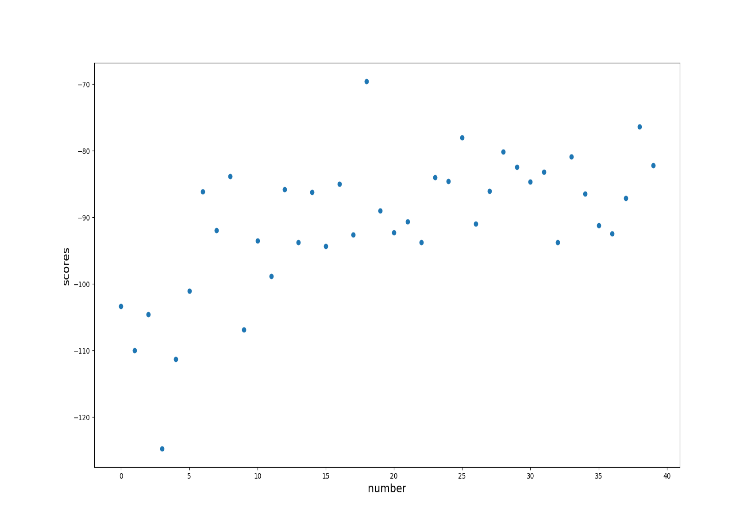
图1. 40个硬件配置的评分结果

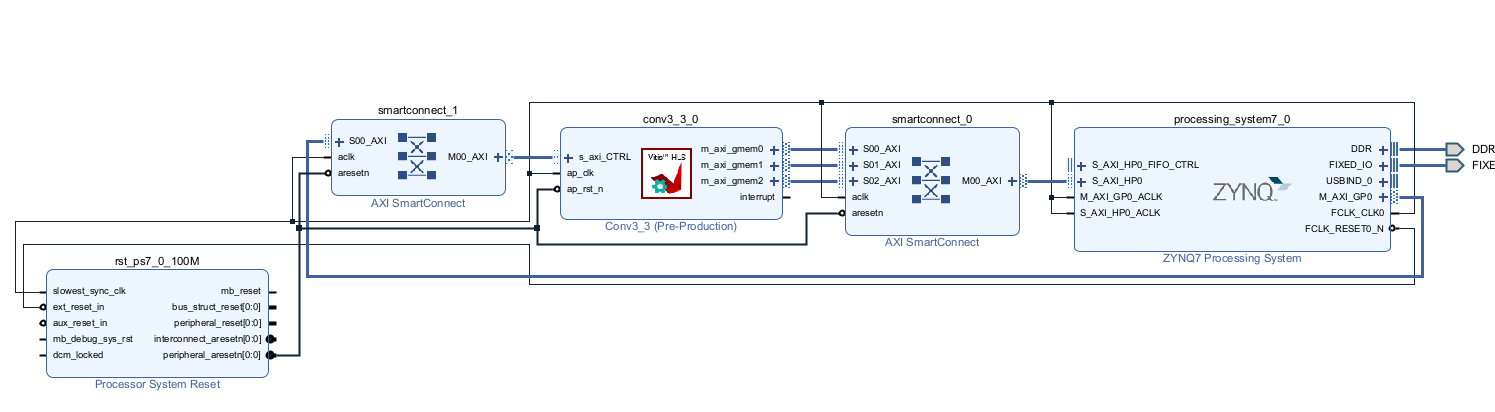                         图2. Vivado中PS和PL连接示意图，采用m_axi模式

       

        利用加速器加速VGG16网络的第10层，进行图像的分类。分别在CPU和CPU-FPGA（FPGA加速）上运行，得到分类结果Top5和预测概率，进行比较，结果如表2所示。

CPU		CPU-FPGA
Top5标签	Top5概率	Top5标签	Top5概率
277	0.926	277	0.909
278	0.026	274	0.032
274	0.021	273	0.029
273	0.018	278	0.024
104	0.005	104	0.003

      表2. FPGA和CPU运行结果比较

3 总结

        结果表明，该卷积核可以正确完成神经网络卷积层的运行，和CPU端的运行结果几乎一致，说明该加速器实现正确。但运行时间仍然较长，这是由于测试的代码是单通道输入，已经做了数据重用，但没有流水线化，没有利用并行计算的优势，同时带宽有限。而第二阶段的DSE的作用就是找出最佳的划块因子，片上网络模板，数据访问和重用模式，提高DNN加速器的性能。本文并没有检测多通道和PE并行优化的HLS模板，并没有实现FPS为30.79，说明该单通道加速器实现性能较差，仍然需要优化。

        同时，遗传算法能够有效的在大量硬件配置中剔除表现差和得分低的配置，从而找到最优配置，提高了搜索的效率。

PYNQ端的运行代码

import numpy as np
#import torch
#import torchvision.models as models
from pynq import Overlay, allocate

# 加载参数
input_feature = np.load("vgg16_input.npy")[0]      # (128,58,58)
weight_tensor = np.load("vgg16_weight.npy")        # (256,128,3,3)

# FPGA 卷积加速
overlay = Overlay("conv_ip.bit")
ip = overlay.conv3_3_0

input_buf = allocate(shape=(128, 58, 58), dtype=np.int32)
weight_buf = allocate(shape=(256, 128, 3, 3), dtype=np.int32)
output_buf = allocate(shape=(256, 56, 56), dtype=np.int32)

scale = 256.0  # 可根据实际调整
input_buf[:] = np.clip((input_feature * scale).round(), -2**31, 2**31-1).astype(np.int32)
weight_buf[:] = np.clip((weight_tensor * scale).round(), -2**31, 2**31-1).astype(np.int32)

print(input_buf)
print(weight_buf)
input_buf.flush()
weight_buf.flush()
output_buf.flush()

ip.write(0x10, input_buf.device_address & 0xFFFFFFFF)
ip.write(0x14, (input_buf.device_address >> 32) & 0xFFFFFFFF)
ip.write(0x1C, weight_buf.device_address & 0xFFFFFFFF)
ip.write(0x20, (weight_buf.device_address >> 32) & 0xFFFFFFFF)
ip.write(0x28, output_buf.device_address & 0xFFFFFFFF)
ip.write(0x2C, (output_buf.device_address >> 32) & 0xFFFFFFFF)

ip.write(0x00, 0x01)
while not (ip.read(0x00) & 0x2):
    pass

output_buf.invalidate()
output_float = output_buf.copy().astype(np.float32) / (scale ** 2)

#x = torch.tensor(output_buf.copy()).unsqueeze(0).float()  # (1,256,56,56)
np.save("vgg16_conv_output.npy", output_float)
# 继续 VGG 推理后半部分

import torch
import torchvision.models as models
import torchvision.transforms as transforms
from PIL import Image
import numpy as np
import torch.nn.functional as F

def preprocess(img_path):
    transform = transforms.Compose([
        transforms.Resize(256),
        transforms.CenterCrop(224),
        transforms.ToTensor(),  # (C,H,W)
        transforms.Normalize(mean=[0.485, 0.456, 0.406],
                             std=[0.229, 0.224, 0.225])
    ])
    img = Image.open(img_path).convert('RGB')
    return transform(img).unsqueeze(0)  # shape: (1, 3, 224, 224)

def extract_input_and_weight_vgg16():
    model = models.vgg16(pretrained=True).eval()
    input_tensor = preprocess("test.jpg")

    # 截取前面直到 features[14] 的子网络（输出 shape 为 (1,128,58,58)）
    partial = torch.nn.Sequential(*list(model.features.children())[:10])
    with torch.no_grad():
        mid_input = partial(input_tensor)
    mid_input_padded = F.pad(mid_input, (1, 1, 1, 1), mode='constant', value=0)  # (1, 128, 58, 58)
    print("中间层输入 shape:", mid_input_padded.shape)  

    # 获取下一层的卷积权重，即 features[15] (Conv2d)
    conv_layer = model.features[10]
    weight = conv_layer.weight.detach().cpu().numpy()

    np.save("vgg16_input.npy", mid_input_padded.cpu().numpy())
    np.save("vgg16_weight.npy", weight)

    print("✅ 已保存输入与权重，送入 FPGA 加速模块")
    return model, mid_input_padded[0], weight  

model, mid_input, weight_tensor = extract_input_and_weight_vgg16()

import numpy as np
import torch
import torchvision.models as models
x0 = np.load("vgg16_conv_output.npy")
print(x0)

x = torch.tensor(x0.copy()).unsqueeze(0).float()  # (1,256,56,56)
# 继续 VGG 推理后半部分
model = models.vgg16(pretrained=True).eval()
back_part = torch.nn.Sequential(*list(model.features.children())[11:])
x = back_part(x)

x = model.avgpool(x)
x = torch.flatten(x, 1)
x = model.classifier(x)

# Top-5
prob = torch.nn.functional.softmax(x, dim=1)[0]
top5 = torch.topk(prob, 5)
print("🎯 Top-5 Prediction:", top5.indices.tolist())
print("🔥 Top-5 Probabilities:", top5.values.tolist())

参考文献

[1] Yongan Zhang, Xiaofan Zhang et al. AutoAI2C: An Automated Hardware Generator for DNN Acceleration on Both FPGA and ASIC[J]. IEEE Transactions on Computer-aided Design of Integrated Circuits and Systems, vol. 43, no. 10, October 2024.

[2] Yu-Hsin Chen et al. Eyeriss v2: A Flexible Accelerator for Emerging Deep Neural Networks on Mobile Devices[J].IEEE Journal on Emerging and Selected Topics in Circuits and Systems, 2019.

[3] https://github.com/tilmto/autoai2c

注：需要在conv3x3.cpp修改接口定义如下：

void conv3_3(data_type* flatten_input, data_type* flatten_weight, data_type* flatten_output ){
#pragma HLS INTERFACE m_axi port=flatten_input depth=430592 offset=slave bundle=gmem0
#pragma HLS INTERFACE m_axi port=flatten_weight depth=294912 offset=slave bundle=gmem1
#pragma HLS INTERFACE m_axi port=flatten_output depth=802816 offset=slave bundle=gmem2

#pragma HLS INTERFACE s_axilite port=flatten_input bundle=CTRL
#pragma HLS INTERFACE s_axilite port=flatten_weight bundle=CTRL
#pragma HLS INTERFACE s_axilite port=flatten_output bundle=CTRL
#pragma HLS INTERFACE s_axilite port=return bundle=CTRL

同时，在input_buffer,output_buffer,weight_buffer函数中加入 #pragma HLS INLINE off

void input_buffer1(data_type input_buffer[0][58][6], data_type* flatten_input,
		          unsigned int ch_in_1, unsigned int o_col, unsigned int o_col_buffer_index){
    	#pragma HLS INLINE off
	for (unsigned int i=0; i<58; i++){
		#pragma HLS PIPELINE
        unsigned int in_col = o_col + 6;
        if (in_col < 58) {
             input_buffer[0][i][o_col_buffer_index] = flatten_input[ch_in_1*58*58 + i*58 + in_col];
         } else {
            input_buffer[0][i][o_col_buffer_index] = 0;  // padding
            }
		//input_buffer[0][i][o_col_buffer_index]=flatten_input[ch_in_1*58*58+i*58+o_col+6];
		}
}